Math Lesson 15.2.1 - Using Simple Factorisation to Plot Quadratic Graphs

Please provide a rating, it takes seconds and helps us to keep this resource free for all to use

Welcome to our Math lesson on Using Simple Factorisation to Plot Quadratic Graphs, this is the first lesson of our suite of math lessons covering the topic of Quadratic Graphs Part Two, you can find links to the other lessons within this tutorial and access additional Math learning resources below this lesson.

Using Simple Factorisation to Plot Quadratic Graphs

In chapter 6 and chapter 9, we explained that quadratic equations with one variable

can be solved by factorising the left part to show it as a product of two expressions in the brackets. This can only be done in two cases out of three possible scenarios.

Case 1: When the quadratic equation has two distinct roots (i.e. when the discriminant Δ is positive). In this case, the above equation is written in the form

where

When the task is to plot the graph of a quadratic equation with two variables

we ignore the existence of variable y first and try to factorise the part containing variable x according to the above rules. The factorisation allows us to find the x-intercepts, as each solution corresponds to an x-intercept. We write the factorised form of a quadratic equation with two variables as

and when solving it, we take y = 0 and write

where x₁ and x² are the solutions (roots) of the quadratic equation with one variable, which correspond to the x-intercepts of the same quadratic equation but with two variables when shown in a graph.

The rest of the points are identified in the same way as when using the quadratic formula to find the roots, exactly as we did in the previous tutorial. Let's see an example to clarify this point.

Example 1

Plot the graph of the following quadratic equation using the factorising method.

Solution 1

We have a = 2, b = 7 and c = 3. Given the relations

and

we obtain

and

Thus, combining the above equations yields p = 1, q = 2, m = -3 and n = -1. Therefore, the factorised equation is

or

Therefore, at the points where the x-intercepts are, we have (x_A - 3) = 0, so x_A = -3, or (2x_B + 1) = 0, so x_B = -1/2.

The corresponding y-values (we expect them to be both zero) are

and

The two x-intercepts therefore are A(-3, 0) and B(-1/2, 0).

As we said in theory, the rest of the solution is the same as in previous examples. Thus, the x-coordinate of the vertex V is

As for the y-coordinate of the vertex, we substitute the above value in the original equation. Thus,

Thus, we have V(-7/4, -25/8).

The y-intercept (for x = 0) is y_C = 3. Therefore, the y-intercept is at C(0, 3).

In the same way as before, we also find the symmetrical point D of the y-intercept. Thus, from the half-line segment formula, where x_V is the midpoint of CDX, we obtain

Thus, we have D(-7/2, 3).

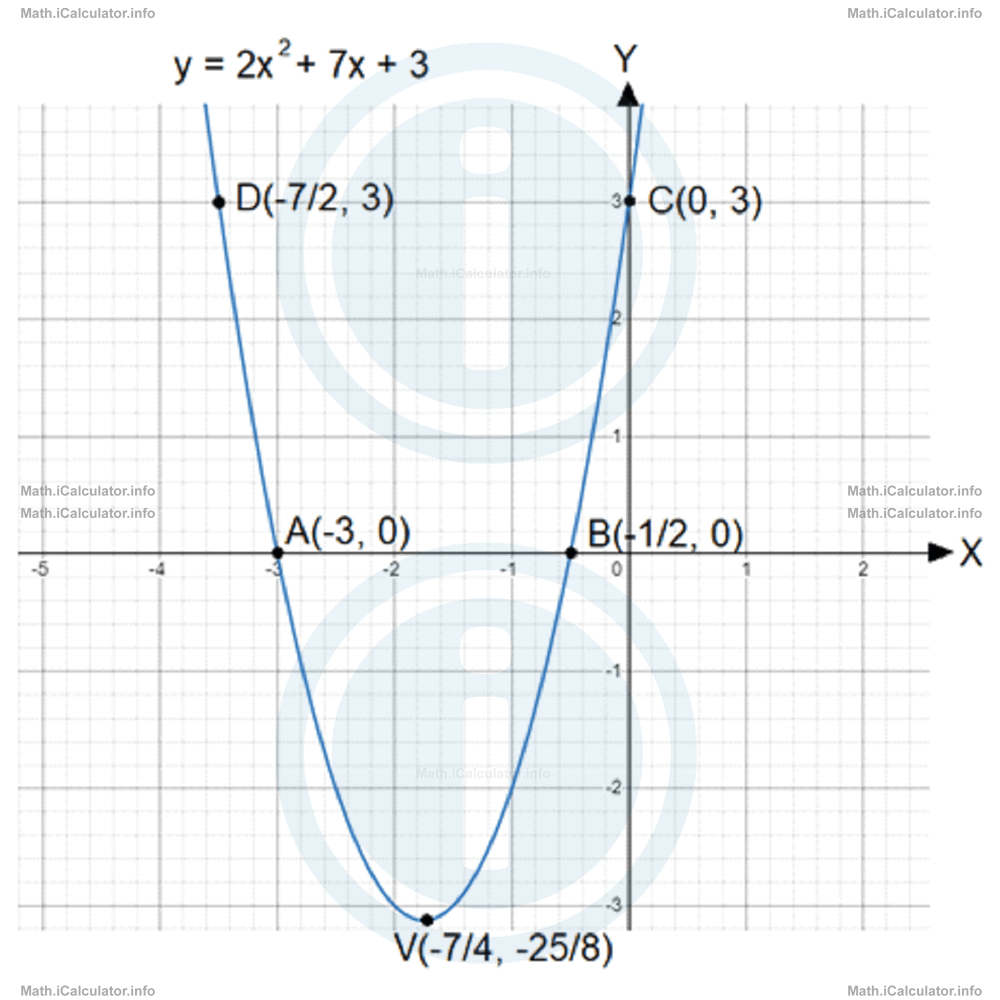
Now, let's plot the graph using the five points found above, i.e. A(-3, 0), B(-1/2, 0), C(0, 3), D(-7/2, 3) and V(-7/4, -25/8).

Case 2: When the quadratic equation has a single root (when the discriminant Δ is zero). In that case, the part containing the independent variable can be written as a binomial expression, so the equation is written in the form

where m is a coefficient and n is a constant.

The corresponding quadratic equations with one variable of the type

have a single solution (root) of the form

Let's see what is the relationship between the original coefficients and constant a, b and c with the new ones, m and n. Thus, since the original form of the quadratic equation with two variables is

and given that we can express the new factorised form as

then we have

In this way, we can find the coefficient m and the constant n if we are convinced that the original quadratic equation has a single root.

Why do we need all this? Well, having a single solution means having a single contact point with the X-axis, which corresponds to the vertex V. Look at the figure below, where the graph of the quadratic equation y = x² - 4x + 4 is shown. It does not take much to prove that this quadratic equation's factorised form is y = (x - 2)².

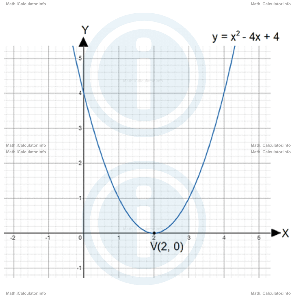
The only solution of the corresponding quadratic equation with one variable x² - 4x + 4 = 0 is x = 2, which corresponds both to the x-intercept and the vertex V.

The question that arises here is: Where to find the other points needed for the graph? Well, like in other cases discussed earlier in the previous tutorial when there were no x-intercepts or when the quadratic graph had a single x-intercept, after finding the vertex you can choose two points on both sides of the vertex that have the same horizontal distance from it and find their y-coordinates. These points have the same effect as the x-intercepts when the parabola intercepts the graph in two different positions. Likewise, we can still use the y-intercept and its symmetrical point concerning the vertical line drawn from the vertex, as we have done in all the other cases discussed in the previous tutorial.

Example 2

Plot the graph of the quadratic equation

using the factorisation method.

Solution 2

We have

Therefore, the only point where the graph intercepts the x-axis is at

which corresponds to the vertex V(1, 0).

Let's find the y-intercept now. Thus, for x = 0, we have y = 4. Therefore, point C(0, 4) is the y-intercept.

The symmetrical point to C is point D with coordinates D(2, 4). This is because the vertex is at x = 1, and given the formula of segment midpoint

we obtain after substituting the known values

It is also known from previous examples that point D has the same y-coordinates as point C. Hence, we have D(2, 4).

We can also find two points A and B equidistant from the vertex in the horizontal direction on both of its sides. For example, since x_V = 1, we can choose x_A = -1 and x_B = 3. The corresponding y-values are

and

Therefore, we have A(-1, 16) and B(3, 16).

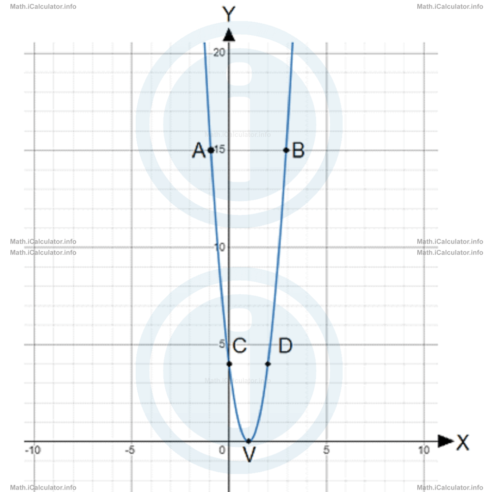
Next, we insert all the five points found above: A(-1, 16), B(3, 16), C(0, 4), D(2, 4) and V(1, 0) in the coordinates system and plot the graph by connecting them smoothly.

Case 3: When the discriminant is negative, there are no x-intercepts at all, so, it is impossible to factorise the expression containing the independent variable. Therefore, we use the same procedure as above to find the necessary points to sketch the graph. Thus, first, we find the vertex V, then the point C that corresponds to the y-intercept, then its symmetrical point D, and at the end, two equidistant points from the vertex: one on its left and the other on its right side. Then, we plot the graph based on these five points.

Example 3

Plot the graph of the quadratic equation

Solution 3

We have a = -1, b = 3 and c = -4. The discriminant Δ is

Since the discriminant is negative, the parabola has no x-intercepts. It has a maximum at the vertex V, which is below the X-axis. First, we find where the vertex V is situated. Its x-coordinate is

Since the discriminant is negative, we cannot use the standard formula of the y-coordinate of the vertex but simply substitute the x-coordinate of the vertex in the main equation. Thus,

Hence, we have V(3/2, -7/4).

Next, let's find the y-intercept C. We already know that x_C = 0, so substituting this value in the main equation yields y_C = -4. Therefore, we have C(0, -4).

Using the segment midpoint formula we can also find the symmetrical point to C, which we denote by D as usual. We have

We know that the y-coordinate of point D is the same as that of C, so we have D(3, -4).

Now, let's find two other symmetrical points A and B on either side of the vertex to complete the set of the necessary points to plot the graph. Since the x-coordinate of the vertex is a fraction, for simplicity we add and subtract it with another fraction, say 5/2, to obtain whole numbers. Therefore, we obtain

and

The corresponding y-values are:

and

(as expected). Therefore, the last two points are A(-1, -8) and B(4, -8).

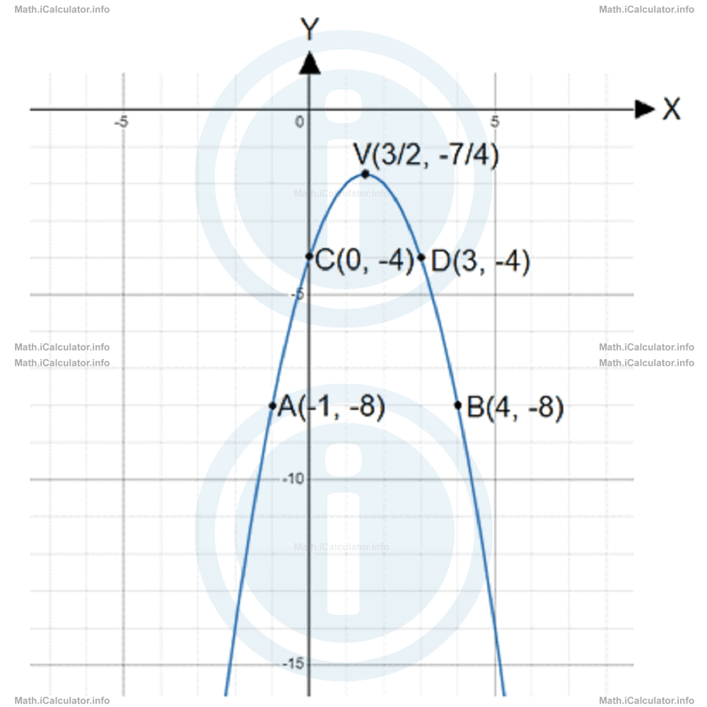
Hence, inserting in the coordinates system all the five points found above: A(-1, -8), B(4, -8), C(0, -4), D(3, -4) and V(3/2, -7/4), yields the following graph after connecting the points smoothly:

You have reached the end of Math lesson 15.2.1 Using Simple Factorisation to Plot Quadratic Graphs. There are 2 lessons in this physics tutorial covering Quadratic Graphs Part Two, you can access all the lessons from this tutorial below.

More Quadratic Graphs Part Two Lessons and Learning Resources

Whats next?

Enjoy the "Using Simple Factorisation to Plot Quadratic Graphs" math lesson? People who liked the "Quadratic Graphs Part Two lesson found the following resources useful:

1. Factorisation Feedback. Helps other - Leave a rating for this factorisation (see below)
2. Types of Graphs Math tutorial: Quadratic Graphs Part Two. Read the Quadratic Graphs Part Two math tutorial and build your math knowledge of Types of Graphs
3. Types of Graphs Revision Notes: Quadratic Graphs Part Two. Print the notes so you can revise the key points covered in the math tutorial for Quadratic Graphs Part Two
4. Types of Graphs Practice Questions: Quadratic Graphs Part Two. Test and improve your knowledge of Quadratic Graphs Part Two with example questins and answers
5. Check your calculations for Types of Graphs questions with our excellent Types of Graphs calculators which contain full equations and calculations clearly displayed line by line. See the Types of Graphs Calculators by iCalculator™ below.
6. Continuing learning types of graphs - read our next math tutorial: Cubic Graphs

Help others Learning Math just like you

Please provide a rating, it takes seconds and helps us to keep this resource free for all to use

We hope you found this Math tutorial "Quadratic Graphs Part Two" useful. If you did it would be great if you could spare the time to rate this math tutorial (simply click on the number of stars that match your assessment of this math learning aide) and/or share on social media, this helps us identify popular tutorials and calculators and expand our free learning resources to support our users around the world have free access to expand their knowledge of math and other disciplines.

Types of Graphs Calculators by iCalculator™