Math Lesson 9.7.3 - Solving Systems of Linear Equations

Please provide a rating, it takes seconds and helps us to keep this resource free for all to use

Welcome to our Math lesson on Solving Systems of Linear Equations, this is the third lesson of our suite of math lessons covering the topic of Systems of Linear Equations. Methods for Solving Them., you can find links to the other lessons within this tutorial and access additional Math learning resources below this lesson.

Methods for Solving Systems of Linear Equations

There are three methods for solving a system of linear equations, where two of which are numerical methods and the third one is graph - based. We will explain each of them in the following part of this tutorial.

1. Elimination method

This is the easiest method for solving linear equations if the proper conditions are met. It consists of the elimination of one of the variables through the addition of the two equations to each other. Creating the proper conditions means multiplying one or both equations by suitable coefficients, to create possible solutions to cancel the variable we choose to eliminate from the resulting equation. Then, we continue with the solution because the new equation obtained, now has only one variable. After calculating the value of this variable, we substitute it in any of the original equations to find the value of the other variable (the one that was eliminated before).

Let's clarify this point through a couple of examples.

Example 3

Solve the following system of linear equations by the elimination method.

Solution 3

We have two choices for eliminating one of the variables:

1. Multiplying by - 3 the first equation only. In this way, we eliminate the variable x after adding the two equations.
2. Multiplying the by 2 the first equation and by - 3 the second equation. In this way, we eliminate the variable y after adding the two equations.

Let's choose the first option. Thus, multiplying the first equation by - 3 yields

Adding the two equations means adding the left sides and the right sides separately. This eliminates the variable x because -3x + 3x = 0 and yields for the rest

Now, we can substitute this value found for y in any of the original equations, for example in the first one. Thus,

Thus, the number pair (5, 3) is a solution set for this system of linear equations.

Proof:

Sometimes, it is necessary to multiply both equations by different coefficients to eliminate any variable, as we will see in the next example.

Example 4

Solve the following system of equations using the elimination method.

Solution 4

First, we must write each equation in the form ax + by = -c. Thus,

Now, let's multiply the first equation by 3 and the second equation by 4 to eliminate y. Thus,

Adding the two equations yields

Let's substitute this value in the first equation to find y (we substitute the value of x in the first equation as it has smaller numbers, but you can substitute it in the second equation as well if you wish). Thus,

Proof:

2. Substitution method

This is the second method for solving a system of linear equations. It consists of choosing an equation from the system for expressing one of the variables in terms of the other variable and then, substituting the corresponding expression in the other equation. In this way, we obtain a first - order equation with one variable.

For example, in the system of equations

we can write the variable y in terms of the other variable x in the first equation, i.e. y = 2x - 5 and substitute the variable y in the second equation with this expression obtained from the first. In this way, we obtain

As for the value of y, we write

Proof:

and

Example 5

Solve the following system of linear equations by substitution method.

Solution 5

It is better to multiply the first equation by 3 first, to eliminate the fraction. Doing this, yields

From the first equation, we obtain y = 3x - 18. We substitute y with this expression into the second equation and solve it for x. Hence,

Now, we can replace the variable x with 10 in any of the equations of the system - for example in the first - to obtain

Proof:

and

Remark! It is not necessary to make the proof after every system you solve. It is recommended however that you make a quick mental proof to be sure that you have correctly solved the system.

3. Graphing method

This method consists of plotting the graphs of each linear equation in the system and checking the coordinates of the meeting point, as they represent the solution set of the system. This is because at the meeting point both equations have the same values for the variable x and also for the other variable y.

We discussed some linear equation graphs in the initial part of this tutorial. We explained that we need to have only two points for each equation given in order to plot the graph of linear equations. We will continue in this way in this part of the tutorial as well.

Let's take an example for illustration. In the system of linear equations

we have to plot the graphs of each equation in the same figure and see where they meet. But first, we have to find two points from each graph that allow us to plot them. We have to choose the values of the x-variable and find the corresponding values of the y-variable. Thus, in the first equation let's take for example x = 0 and x = 2. Substituting them in the first equation we obtain

and

Therefore, points A(0, 5) and B(2, 9) are points that belong to the first graph.

Then, we follow the same procedure for the second equation of the system as well. We can take x = -5 and x = 4 and find the corresponding y-values. Thus,

and

Therefore, points C( - 5, 0) and D(4, 3) are points that belong to the first graph.

Now, we plot both graphs in the same coordinate system as shown below.

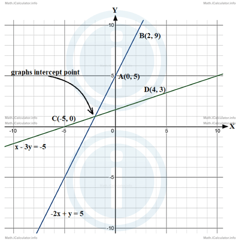
As you see, the intercept point is at ( - 2, 1). This means the solution set of this system of equations is x = -2 and y = 1.

We can confirm this graphical solution through one of the other methods discussed earlier; for example through the elimination method. Thus, multiplying by 3 the first equation of the system

to eliminate y, yields

Adding the two equations, yields

Hence, substituting this value in the second equation (for convenience) yields

These results are identical to those obtained through the graphing method.

Example 6

Solve the following system of linear equations through the graphing method.

Solution 6

We can create tables to have the values arranged better. Thus,

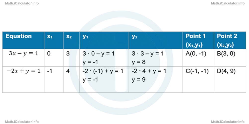
Hence, the graphs of the two equations are as shown below:

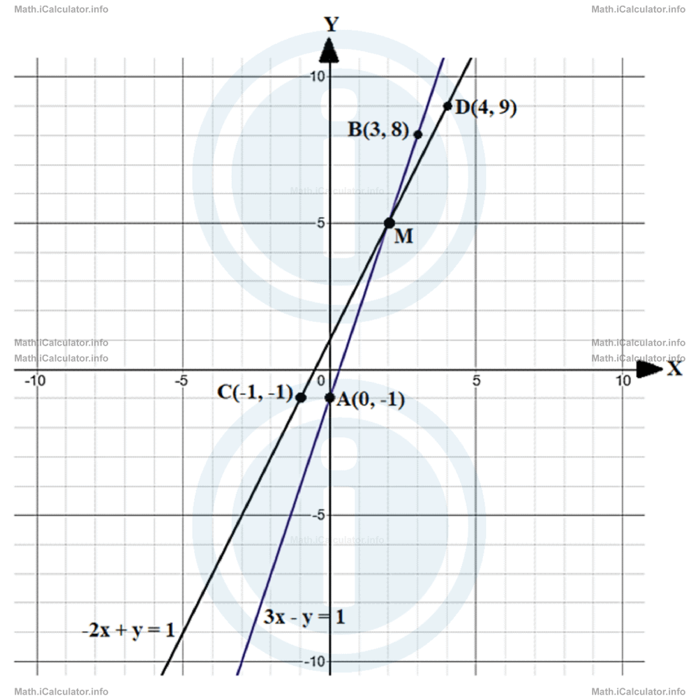vFrom the figure, it is clear that point M is the intercept of the two lines. It has the coordinates M(2, 5). This means the solution set of our system of equations is x = 2 and y = 5. We can prove this solution by replacing the variables with these values in the system. Thus, for the first equation, we have

and for the second equation, we have

More Systems of Linear Equations. Methods for Solving Them. Lessons and Learning Resources

Equations Learning Material

Tutorial ID	Math Tutorial Title	Tutorial	Video Tutorial	Revision Notes	Revision Questions
9.7	Systems of Linear Equations. Methods for Solving Them.
Lesson ID	Math Lesson Title			Lesson	Video Lesson
9.7.1	Linear Equations Definition
9.7.2	Systems of Linear Equations
9.7.3	Solving Systems of Linear Equations

Whats next?

Enjoy the "Solving Systems of Linear Equations" math lesson? People who liked the "Systems of Linear Equations. Methods for Solving Them. lesson found the following resources useful:

1. Solving Systems Feedback. Helps other - Leave a rating for this solving systems (see below)
2. Equations Math tutorial: Systems of Linear Equations. Methods for Solving Them.. Read the Systems of Linear Equations. Methods for Solving Them. math tutorial and build your math knowledge of Equations
3. Equations Video tutorial: Systems of Linear Equations. Methods for Solving Them.. Watch or listen to the Systems of Linear Equations. Methods for Solving Them. video tutorial, a useful way to help you revise when travelling to and from school/college
4. Equations Revision Notes: Systems of Linear Equations. Methods for Solving Them.. Print the notes so you can revise the key points covered in the math tutorial for Systems of Linear Equations. Methods for Solving Them.
5. Equations Practice Questions: Systems of Linear Equations. Methods for Solving Them.. Test and improve your knowledge of Systems of Linear Equations. Methods for Solving Them. with example questins and answers
6. Check your calculations for Equations questions with our excellent Equations calculators which contain full equations and calculations clearly displayed line by line. See the Equations Calculators by iCalculator™ below.
7. Continuing learning equations - read our next math tutorial: Relationship between Equations in Linear Systems. Systems of Equations with One Linear and One Quadratic Equation

Help others Learning Math just like you

Please provide a rating, it takes seconds and helps us to keep this resource free for all to use

We hope you found this Math tutorial "Systems of Linear Equations. Methods for Solving Them." useful. If you did it would be great if you could spare the time to rate this math tutorial (simply click on the number of stars that match your assessment of this math learning aide) and/or share on social media, this helps us identify popular tutorials and calculators and expand our free learning resources to support our users around the world have free access to expand their knowledge of math and other disciplines.

Equations Calculators by iCalculator™

• Completing The Square In Quadratics Calculator
• First Order Equations With One Variable Calculator
• First Order Equations With Two Variables Calculator
• Solving Quadratics Through The Quadratic Formula
• Solving Systems Of Linear Equations With The Substituting Method Calculator
• Solving Systems With One Linear And One Quadratic Equation Calculator