Math Lesson 15.3.2 - Features of Cubic Graphs

Please provide a rating, it takes seconds and helps us to keep this resource free for all to use

Welcome to our Math lesson on Features of Cubic Graphs, this is the second lesson of our suite of math lessons covering the topic of Cubic Graphs, you can find links to the other lessons within this tutorial and access additional Math learning resources below this lesson.

Features of Cubic Graphs

Cubic graphs have some features that are specific only for them. Below, we will discuss these features illustrated with examples.

1. The wiggles

A common feature of all cubic graphs is a kind of 'wiggle' - a change in the form of the curve that lies around the point where the graph changes shape. Look at the figure below.

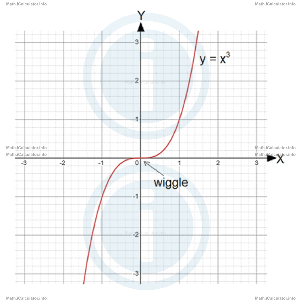
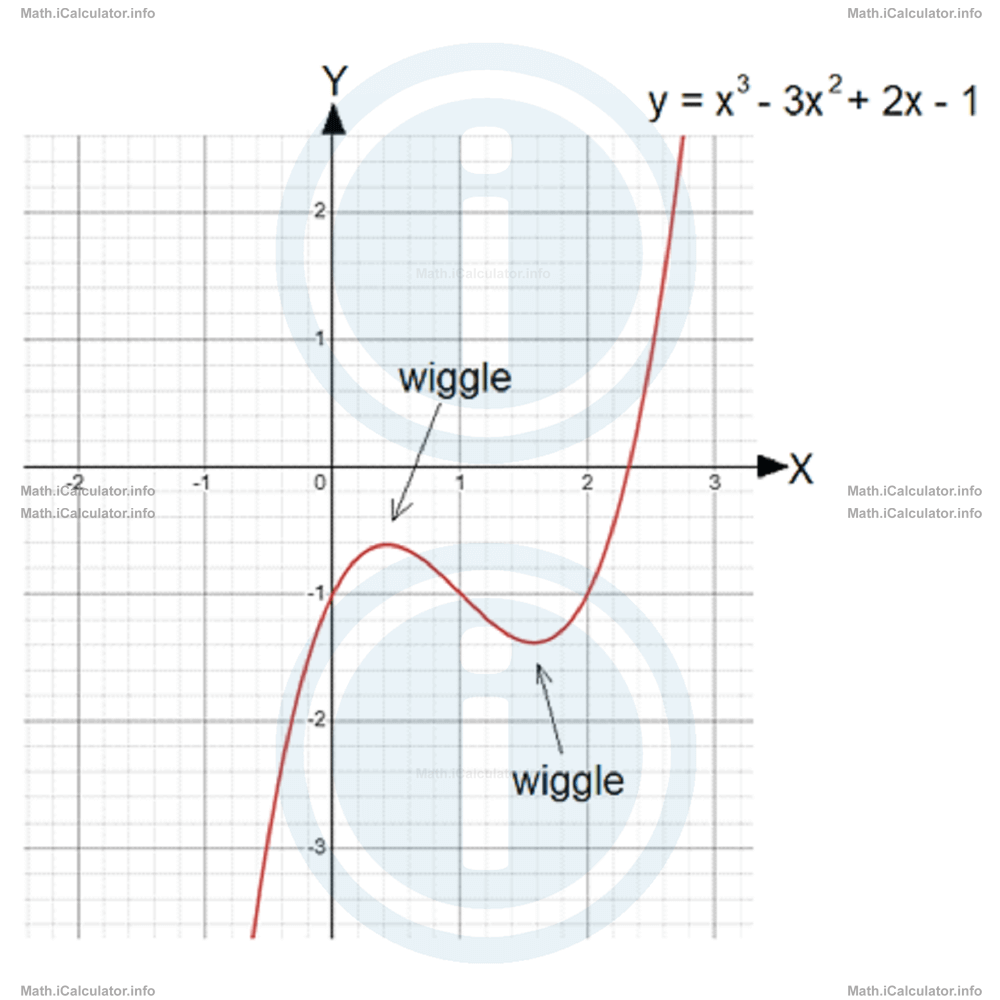
The above graph shows the simplest form of a cubic graph resulting from the simplest form of the cubic functions, y = x³, where all coefficients and the constant are zero except the coefficient a, which is 1. However, in more complex cubic functions there may be more than one wiggle, as shown in the figure below.

Wiggles have special names in mathematics, which we will explain later. For now, it is enough to highlight their importance consisting of two main elements:

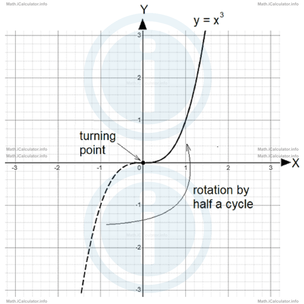
1. If the cubic graph has a single wiggle, then its central point is a kind of turning point for the graph which produces some symmetry in the sense that, if you rotate by half a cycle one of the 'arms' of the graph, it will fit with the other arm of the same graph.
2. If the cubic graph has more than one wiggle, then each of these wiggles represents a local minimum or maximum for the corresponding cubic function.

They are called 'local' because the absolute minimum and maximum are minus and plus infinity respectively, given that the graph goes towards the minus infinity on one side and towards the plus infinity on the other. (With maximum or minimum, we mean the y-values of the given points). For example, the cubic graph above has a local maximum slightly smaller than 1 and a local minimum slightly smaller than -4.

Example 1

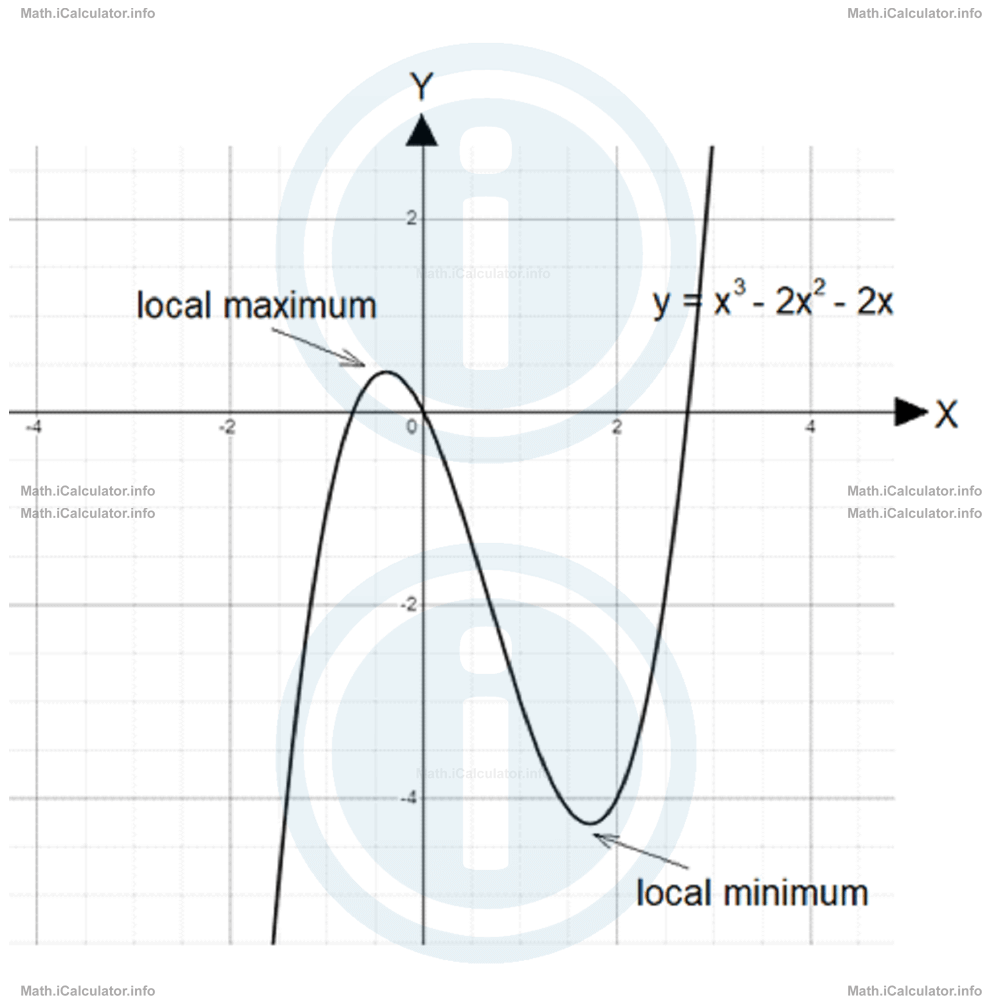
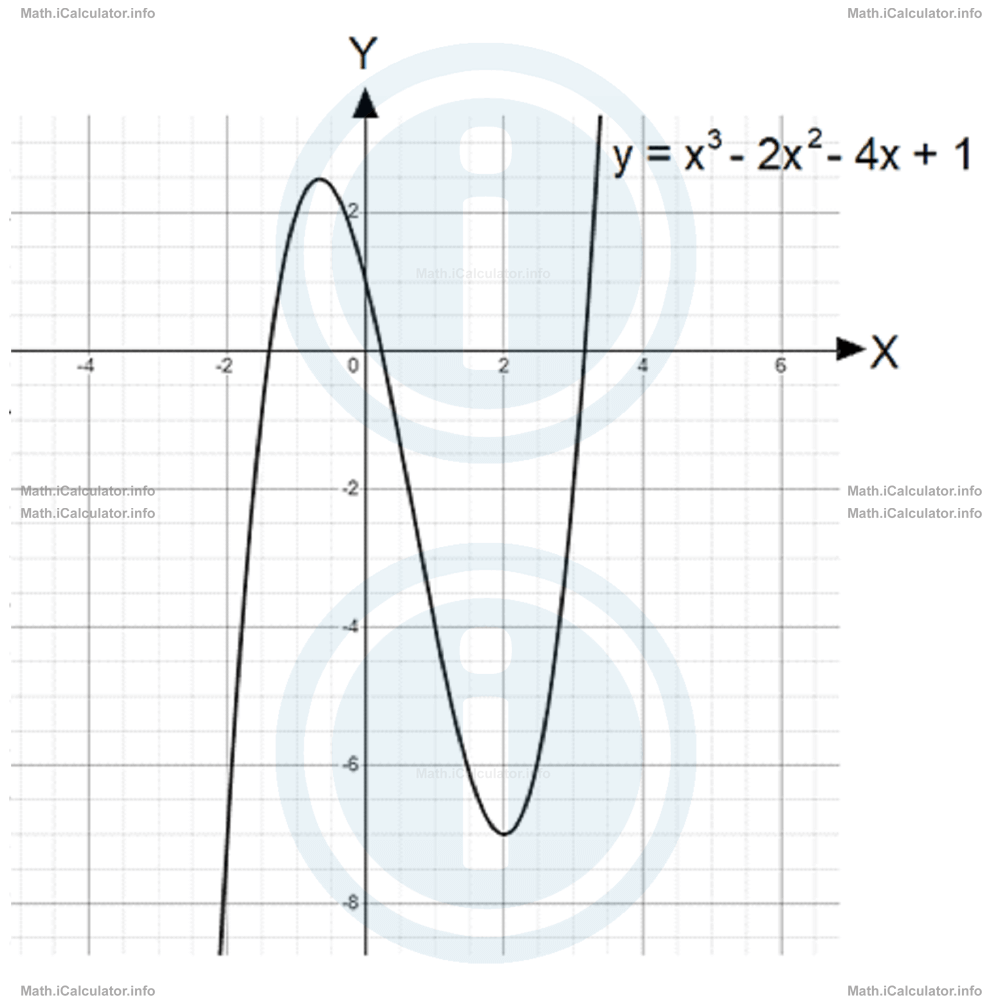
From the figure below, identify the coordinates of the local maximum and local minimum of the graph.

Solution 1

From the figure, it is obvious that the graph has a local maximum and a local minimum. The question requires us to find both coordinates for the two points identified. The y-values of these points are identified simply by sight. Thus, the local maximum is at y = 2.5 (or 5/2) while the local minimum is at y = -7. (The true y-value of the maximum is a little smaller than 2.5 actually, but we rounded it to the nearest tenth of a unit).

The corresponding x-values are normally found by substituting the above y-values in the original equation of the line, but since this equation is in the third power, this is a very challenging task that can be done only by iterative methods. Therefore, at the moment we don't want to use any iterative method but focus only on the graph, the result is x = -2/3 for the x-coordinate of the local maximum and x = 2 for the local minimum. Therefore, the local maximum is at (-2/3, 5/2) while the local minimum is at (2, -7). Look at the figure.

Remark! Actually, all cubic graphs have two wiggles. However, in some of them the local minimum and maximum are hardly detectable, which makes us consider a single wiggle. In fact, this single wiggle is produced by the combination of the two wiggles given that they are almost at the same position. For example, in the cubic graph we considered earlier, which is obtained by the equation y = x³, the two wiggles are almost converging at the turning point and the distinction between them becomes almost invisible.

2. The orientation of the curve

Now, let's focus on the orientation of the curve, i.e. in understanding where the curve comes from on the left side and where it goes on the right side. This depends on the sign of coefficient a. Thus, if coefficient a is positive (a > 0), the graph comes from the bottom left and goes up to the top right, as occurred in all cubic graphs seen so far in this tutorial.

On the other hand, if coefficient a is negative (a < 0), then the cubic graph comes from the top left and goes down to the bottom right side.

Look at the following figure.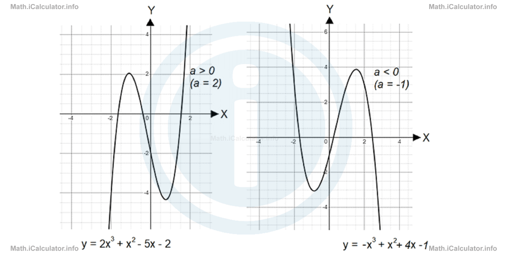

The first graph shows the line y = 2x³ + x² - 5x - 2. Since a = 2 (positive, therefore), the graph comes from the minus infinity on the left side, makes a couple of wiggles and goes towards plus infinity on the right side.

The second graph instead, shows the line y = -x³ + x² + 4x - 1. Since a = - 1 (negative, therefore), the graph comes from the plus infinity on the left side, makes a couple of wiggles and goes towards minus infinity on the right side.

3. The intercepts with the two axes

From the definition of the function given in the previous chapter, it is clear that for every x-value in a function there must be a single y-value that corresponds to a single point on the graph. Cubic graphs are visual representations of cubic functions. Therefore, for every x-value in a cubic graph there is a single corresponding y-value. This means cubic graphs have a single y-intercept obtained for x = 0, similar to quadratic or linear graphs. Hence, since the general form of a cubic equation with two variables (cubic function) is

substituting x = 0, we obtain y = d. Therefore, the y-intercept of a cubic function is at M(0, d).

On the other hand, the x-intercepts are obtained for y = 0. From chapter 9, is known that the maximum number of roots of any equation corresponds to the degree of the polynomial it is made of. For example, a linear equation may have 0 or 1 root, depending on the values of the coefficient (gradient) m and the constant n; a quadratic equation may have 0, 1 or 2 roots, depending on the value of the coefficients a and b and the constant c - values that determine the sign of the discriminant.

In cubic equations, however, there are no such things. We simply know that the y-value must be taken as 0, so the simplified form of this cubic equation (now with a single variable)

is obtained.

We explained in other math tutorials that sometimes it is possible to factorise cubic equations by writing them as a product of two pairs of brackets, where one of them contains a first-degree equation and the other, a quadratic one. This helps us a lot when finding the roots of the equation, which correspond to the x-intercepts. Look at the example below.

Example 2

Find the intercepts of the y = x³ + x² - 4x - 4 with the X- and Y-axes.

Solution 2

First, let's find the y-intercept, as it is easier to calculate. Thus, for x = 0, we have y = -4. Therefore, the point M(0, -4) is the y-intercept of the graph.

As for the x-intercepts, we try to transform the right part of the original equation in a suitable way, to obtain any possible factorisation. In addition, we take y = 0. In this way, we obtain

The first bracket represents an expression of the form a₃ - b₃ (one of the eight special algebraic identities discussed in chapter 6 and chapter 9) where b = 2, which is factorised as (a - b)(a² + ab + b²). Hence, we obtain

As for the second expression in the brackets, it is clear that it represents the expanded form of the binomial (x - 2)₂, given the equivalent transformation

Therefore, we can write the simplified version of the cubic equation (with y = 0) as

We see that (x - 2) is a common part of the two above expressions, so, we factorise it. Thus, we obtain

This equation is true for x - 2 = 0, i.e. for x = 2 (which is one of the x-intercepts) and for x² + 3x + 2 = 0. Solving this new quadratic equation (where the same types of transformations and factorisations as before are involved) yields

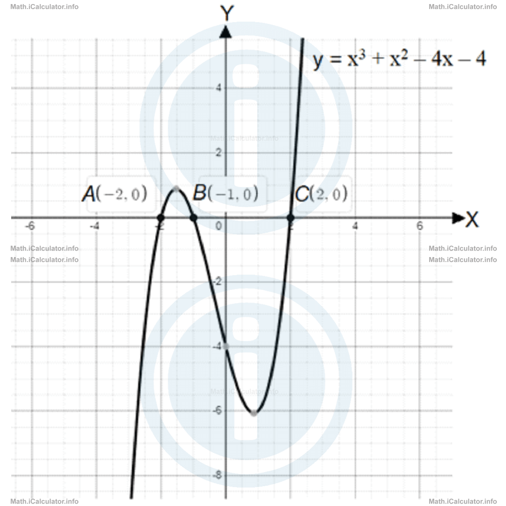
This equation is true for x + 1 = 0 (i.e. for x = -1) and for x + 2 = 0 (i.e. for x = -2). Therefore, the three x-intercepts of the graph are A(-2, 0), B(-1, 0) and C(2, 0).

The above results are confirmed by plotting the graph using any graph-plotting software, as shown below.

Remark! Not all cubic equations can be factorised. Moreover, even if they can be factorised, one of the expressions in the brackets may not have any real root. This makes most of the corresponding cubic equations have less than three roots. Look at the example below.

Example 3

Find the number of x-intercepts of the cubic graph given by the equation

Solution 3

The first thing we can notice from the equation is the common factor 2x. Hence, we can write

Now, let's consider the simplified version of this equation, in which y = 0, to find the roots. Thus, we have

This equation is true for

i.e. for

and for

which we can write as

This equation is true for x = 1.

Therefore, the original equation has two roots: x = 0 and x = 1, which correspond to the x-intercepts of the graph produced by this equation. Hence, the graph has only two x-intercepts: O(0, 0) and A(1, 0).

You have reached the end of Math lesson 15.3.2 Features of Cubic Graphs. There are 3 lessons in this physics tutorial covering Cubic Graphs, you can access all the lessons from this tutorial below.

More Cubic Graphs Lessons and Learning Resources

Whats next?

Enjoy the "Features of Cubic Graphs" math lesson? People who liked the "Cubic Graphs lesson found the following resources useful:

1. Features Feedback. Helps other - Leave a rating for this features (see below)
2. Types of Graphs Math tutorial: Cubic Graphs. Read the Cubic Graphs math tutorial and build your math knowledge of Types of Graphs
3. Types of Graphs Revision Notes: Cubic Graphs. Print the notes so you can revise the key points covered in the math tutorial for Cubic Graphs
4. Types of Graphs Practice Questions: Cubic Graphs. Test and improve your knowledge of Cubic Graphs with example questins and answers
5. Check your calculations for Types of Graphs questions with our excellent Types of Graphs calculators which contain full equations and calculations clearly displayed line by line. See the Types of Graphs Calculators by iCalculator™ below.
6. Continuing learning types of graphs - read our next math tutorial: Reciprocal Graphs

Help others Learning Math just like you

Please provide a rating, it takes seconds and helps us to keep this resource free for all to use

We hope you found this Math tutorial "Cubic Graphs" useful. If you did it would be great if you could spare the time to rate this math tutorial (simply click on the number of stars that match your assessment of this math learning aide) and/or share on social media, this helps us identify popular tutorials and calculators and expand our free learning resources to support our users around the world have free access to expand their knowledge of math and other disciplines.

Types of Graphs Calculators by iCalculator™