Math Lesson 9.4.1 - Iterative Methods for Solving Equations

Please provide a rating, it takes seconds and helps us to keep this resource free for all to use

Welcome to our Math lesson on Iterative Methods for Solving Equations, this is the first lesson of our suite of math lessons covering the topic of Iterative Methods for Solving Equations, you can find links to the other lessons within this tutorial and access additional Math learning resources below this lesson.

What are Iterative Methods for Solving Equations?

When the exact solution of an equation is impossible to find because the roots are real (infinite) numbers, we apply iterative methods consisting of approximate solutions to more complex equations through repeating procedures. The term "iteration" means repeatedly carrying on a process.

In iterative methods, we first make a plan and choose to calculate the root values to a certain degree of accuracy (for example, to the nearest integer, tenth, hundredth, etc.) and then, we apply the procedure as many times as needed to "isolate" the possible solution to the desired order of accuracy. Let's get more in detail about these procedures.

Change of Sign Method

Before explaining the change of sign method to solve equations that have real numbers as roots, let's consider an example consisting of a first - order equation with one variable, which as we know, has a fixed root. Let's consider the equation 3x - 5 = 7. Solving this equation yields

This means that for x = 4 the equation is true, i.e. its left part is equal to zero.

Now, let's suppose we don't know the root of the equation but we are going to guess it by identifying the zone where this root may be present. Let's take x = 1. For this value, we have

For x = 2, we have

For x = 3, we have

As you see, we are getting closer to zero. This means that we are approaching the root value, which is still bigger than 3.

On the other hand, if x = 6, we have

This means we are on the other side of the root, i.e. it is smaller than 6.

For x = 5, we have

As 3 is closer to 0 than 6, this means x = 5 is closer to the true root than x = 6. Therefore, the solution must be searched in the numbers zone that contains values bigger than 3 and smaller than 5, i.e. somewhere around the value 4. (We know that the root is 4, as we have solved this simple equation; this example is used only for illustration purpose of iterative methods.

Again, taking x = 3.9 yields

And for x = 4.1 we have

We can continue this way with x = 3.99 and x = 4.01 (they give - 0.03 and 0.03 respectively). Therefore, it becomes more and more clear that the root of this equation is x = 4.

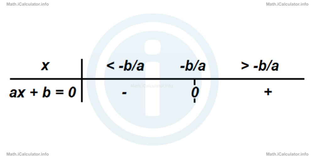
In first - order equations therefore, the root is at the point x = - b/a. For x < -b/a, the sign of the left part of the equation is negative, while for x > - b/a, it is positive.

The sign table of first - order equations is shown below.

Obviously, in first - order equations with one variable, it is not necessary to apply any iterative methods, as it is easier to solve the equation. The utility of such methods is more evident in higher - order equations. Let's explain this point through an example.

Example 1

Find one root of the equation 3x³ - 4x² + x - 1 = 0 (at an accuracy of one decimal place) that is near to the number x = 1.

Solution 1

For x = 1, we have

For x = 1.2, we have

Since we are getting closer to zero, we continue increasing the value of x by small steps. Hence, for x = 1.4, we have

Given that the result is positive, this means that we have gone beyond the root. Therefore, the solution must be searched between x = 1.2 and x = 1.4. Hence, let's try x = 1.3 and eventually see whether the result is closer to - 0.576 or 0.392. Thus, for x = 1.3, we have

Hence, since - 0.169 is closer to zero than - 0.596 and 0.392, we take this value (x = 1.3) as the solution of the original equation if we want to stop at one decimal place.

The iterative method used in the above equations is known as the change of sign method for solving an equation. Thus, according to this method, we must look for the solutions (roots) where the expression contained in the left part of an equation is about to change the sign. The values of an equation's variables for which the corresponding expressions are exactly zero represent the roots (solutions) of this equation. The closer to zero the value of this expression is, the closer to the correct value of the variable is the number chosen to represent the variable in calculations.

There are two 'change of sign' methods we can use when solving an equation through iterative methods. They are:

Method 1: Going through values in order until there is a change in sign.

For example, in the equation

we can start from x = 0 to substitute the variable in the equation. We have

For x = 1, we have

For x = 2, we have

Thus, since there is a change in sign, it is certain that one of the roots of this equation is between 1 and 2. From the results obtained for the corresponding expression, it is clear that the root is much closer to 1 than 2 (as - 5 is much closer to zero than 132). Hence, we may continue with other numbers to get closer to the solution. For example, we can try x = 1.1. Thus,

Again, we continue to increase the accuracy of the result by taking x = 1.2. We have

Hence, we were able to localize more in detail the position of the root. It is between 1.1 and 1.2 (closer to 1.1). If we want to increase the accuracy further, we can take x = 1.11; x = 1.12; etc., unless we obtain again a new change in sign.

Method 2: Using the half - interval division to localize the root.

This means that after identifying an interval where is a change in sign, take half of that interval and make a new calculation. Then, we consider again the half interval where there is a change in sign and consider the half of this half (one - quarter of the original interval), and so on. This procedure is carried out until we obtain the desired level of accuracy.

For example, in the equation

when starting from x = 0, this yields

For x = 1, we have

Since there is a change in sign, the root is between 0 and 1. Thus, we take half of this interval (x = 0.5) and make the calculations again.

Therefore, the solution is between x = 0.5 and x = 1, as the change in sign occurs in this interval. Hence, we take again the half - value, i.e. x = 0.75. Thus,

Since we obtained again a negative value, the solution must be searched in the other half, i.e. between 0.75 and 1. Thus, for x = 0.875, we have

In this way, the root is between 0.75 and 0.875. Therefore, if we want to round the result in one decimal place, we write x = 0.8. If we want to write the result in two decimal places, we must continue further the above procedure until obtaining the desired result.

Example 2

Use the iterative method of half - intervals to find one root of the equation x⁵ - 2x - 2 = 0. Write the answer in one decimal place.

Solution 2

At a first glance, it is clear that one of the possible the solution must be searched between x = 1 and x = 2, as

and

Hence, taking x = 1.5 as half - interval yields

Therefore, the root is less than 1.5 as the change in sign is between 1 and 1.5. Thus, taking the value x = 1.25 for the half - interval yields

This means the result must be searched between 1.25 and 1.5. Thus, for x = 1.375 (the middle point of 1.25 and 1.5), we obtain

Hence, the root is between 1.25 and 1.375. This means that when rounded to one decimal place, the result is x = 1.3.

More Iterative Methods for Solving Equations Lessons and Learning Resources

Whats next?

Enjoy the "Iterative Methods for Solving Equations" math lesson? People who liked the "Iterative Methods for Solving Equations lesson found the following resources useful:

1. Solving Equations Feedback. Helps other - Leave a rating for this solving equations (see below)
2. Equations Math tutorial: Iterative Methods for Solving Equations. Read the Iterative Methods for Solving Equations math tutorial and build your math knowledge of Equations
3. Equations Video tutorial: Iterative Methods for Solving Equations. Watch or listen to the Iterative Methods for Solving Equations video tutorial, a useful way to help you revise when travelling to and from school/college
4. Equations Revision Notes: Iterative Methods for Solving Equations. Print the notes so you can revise the key points covered in the math tutorial for Iterative Methods for Solving Equations
5. Equations Practice Questions: Iterative Methods for Solving Equations. Test and improve your knowledge of Iterative Methods for Solving Equations with example questins and answers
6. Check your calculations for Equations questions with our excellent Equations calculators which contain full equations and calculations clearly displayed line by line. See the Equations Calculators by iCalculator™ below.
7. Continuing learning equations - read our next math tutorial: Quadratic Equations

Help others Learning Math just like you

Please provide a rating, it takes seconds and helps us to keep this resource free for all to use

We hope you found this Math tutorial "Iterative Methods for Solving Equations" useful. If you did it would be great if you could spare the time to rate this math tutorial (simply click on the number of stars that match your assessment of this math learning aide) and/or share on social media, this helps us identify popular tutorials and calculators and expand our free learning resources to support our users around the world have free access to expand their knowledge of math and other disciplines.

Equations Calculators by iCalculator™

• Completing The Square In Quadratics Calculator
• First Order Equations With One Variable Calculator
• First Order Equations With Two Variables Calculator
• Solving Quadratics Through The Quadratic Formula
• Solving Systems Of Linear Equations With The Substituting Method Calculator
• Solving Systems With One Linear And One Quadratic Equation Calculator