Math Lesson 13.3.2 - Exponential Function Graphs

Please provide a rating, it takes seconds and helps us to keep this resource free for all to use

Welcome to our Math lesson on Exponential Function Graphs, this is the second lesson of our suite of math lessons covering the topic of Modelling Curves using Logarithms, you can find links to the other lessons within this tutorial and access additional Math learning resources below this lesson.

Exponential Function Graphs

By definition, an exponential function is a function that has the independent variable in the exponent of one of its terms. The simplest general form of exponential functions is

where 'a' is a constant. More advanced exponential functions include the following forms

where a, b, m and n are all numbers.

Perhaps, the most widespread exponential function is y(x) = em^x, where 'e' is the Euler's number discussed in Tutorial 13.1 (e = 2.71828). However, we will explain and work with these functions in the next tutorial, where we explain natural logarithms.

The graph of an exponential function is a curve that extends to infinity on three sides but has some limitations on the other, depending on the value of the base and the sign of the exponent. The best method to plot the graph of an exponential function is to find as many points of the graph as possible. If the formula of the function is known, we can give some arbitrary values to the independent variable x and then calculate the corresponding y-values.

Based on the above two criteria (base and sign of exponent), we can list the following cases about the exponential function graphs.

1. The base is greater than 1 and the coefficient m before the variable x in the exponent is positive (a > 1 and m > 0). The graph of such functions extends above zero in the vertical axis (y-axis) to infinity. On the other hand, it extends to the infinity on both sides of the horizontal axis (x-axis) but at a faster rate on the left, where it approaches zero. Moreover, the graph is decreasing when moving from left to right. Look at the graph of the function y(x) = 2x (a = 2 and m = 1) shown below for illustration. 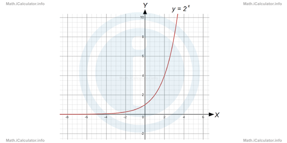This form also includes graphs of the exponential functions such as
   y(x) = a^mx; y(x) = a^{mx + n}; y(x) = b ∙ a^x; y(x) = b ∙ a^mx and y(x) = b ∙ a^{mx + n}
   with the condition that m > 0, n > 0 and b > 1. The only difference is that the graph may be more stretched or compressed laterally, depending on the values of a, b, m and n.
2. The base is greater than 1 and the coefficient m before the variable x in the exponent is negative (a > 1 and m < 0). The graph of such functions extends above zero in the vertical axis (y-axis) to infinity. On the other hand, it extends to the infinity on both sides of the horizontal axis (x-axis) but at a faster rate on the right, where it approaches zero. Moreover, the graph is decreasing when moving from left to right. Look at the graph of the function y(x) = 2 - x (a = 2 and m = -1) shown below for illustration. 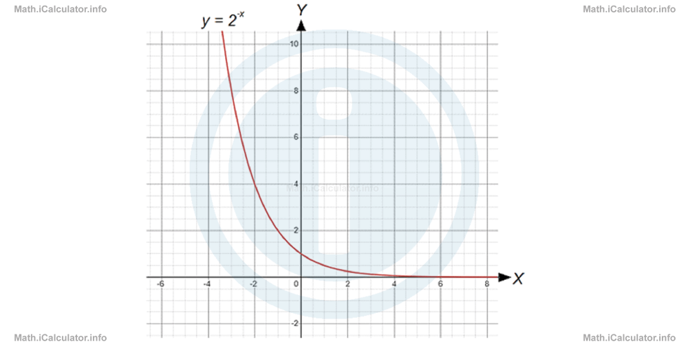This form also includes graphs of the exponential functions such as
   y(x) = a^mx; y(x) = a^{mx + n}; y(x) = b ∙ a^x; y(x) = b ∙ a^mx and y(x) = b ∙ a^{mx + n}
   with the condition that m < 0, n < 0 and b > 1. The only difference is that the graph may be more stretched or compressed laterally, depending on the values of a, b, m and n.
3. The base is smaller than 1 (but greater than 0 anyway) and the coefficient m before the variable x in the exponent is positive (a < 1 and m > 0). By expressing a = 1/c , we can transform such functions in the following way:
   y(x) = a^x = (1/c)^x = (c^-1 )^x = c^-x
   In this way, the graph of this function is similar to that explained in point 2 below, as shown in the figure below. 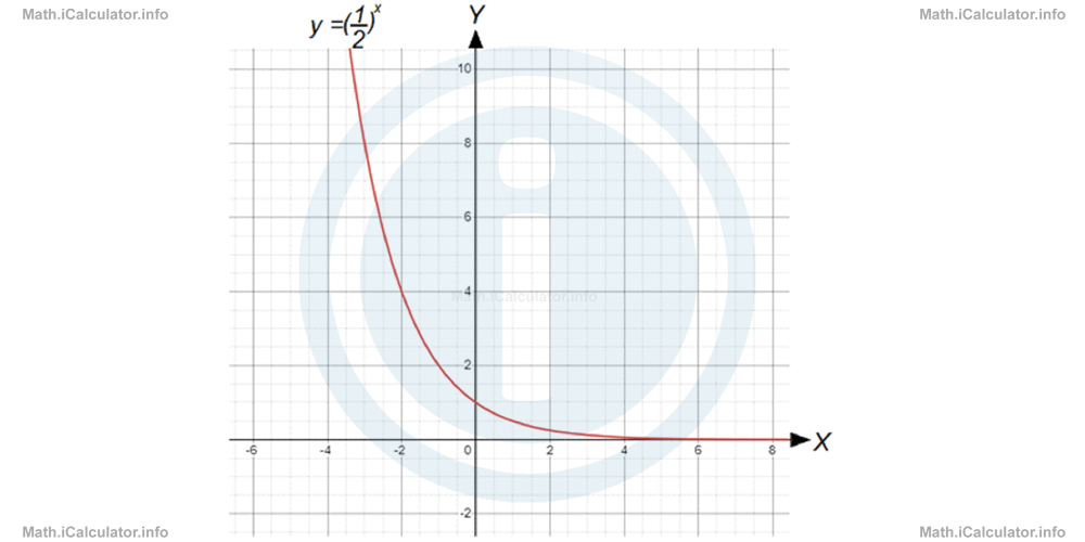This form also includes graphs of the exponential functions such as
   y(x) = a^mx; y(x) = a^{mx + n}; y(x) = b ∙ a^x; y(x) = b ∙ a^mx and y(x) = b ∙ a^{mx + n}
   with the condition that m > 0, n > 0 and b < 1. The only difference is that the graph may be more stretched or compressed laterally, depending on the values of a, b, m and n.
4. Likewise, the graph of the exponential function y(x) = a - x when a < 1 is similar to y(x) = ax when a > 1 (discussed in the first case). Therefore, the graph will also be similar, as shown in the figure below where the graph of the function y = (1/2) - x is plotted. 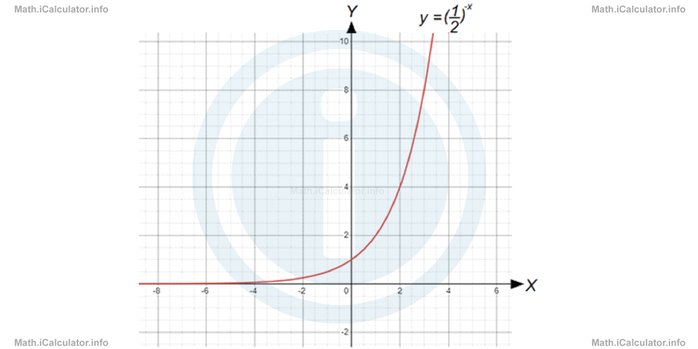This form also includes graphs of the exponential functions such as
   y(x) = a^mx; y(x) = a^{mx + n}; y(x) = b ∙ a^x; y(x) = b ∙ a^mx and y(x) = b ∙ a^{mx + n}
   with the condition that m < 0, n < 0 and b < 1. The only difference is that the graph may be more stretched or compressed laterally, depending on the values of a, b, m and n.

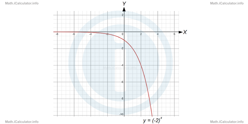
Remark! If a < 0, the graph is inverted down with respect to the graph of the corresponding exponential function with a > 0. For example, the function y(x) = (-2)^x has a similar graph to y(x) = 2^x but inverted down, as shown in the figure below.

More Modelling Curves using Logarithms Lessons and Learning Resources

Whats next?

Enjoy the "Exponential Function Graphs" math lesson? People who liked the "Modelling Curves using Logarithms lesson found the following resources useful:

1. Exponential Function Graphs Feedback. Helps other - Leave a rating for this exponential function graphs (see below)
2. Logarithms Math tutorial: Modelling Curves using Logarithms. Read the Modelling Curves using Logarithms math tutorial and build your math knowledge of Logarithms
3. Logarithms Video tutorial: Modelling Curves using Logarithms. Watch or listen to the Modelling Curves using Logarithms video tutorial, a useful way to help you revise when travelling to and from school/college
4. Logarithms Revision Notes: Modelling Curves using Logarithms. Print the notes so you can revise the key points covered in the math tutorial for Modelling Curves using Logarithms
5. Logarithms Practice Questions: Modelling Curves using Logarithms. Test and improve your knowledge of Modelling Curves using Logarithms with example questins and answers
6. Check your calculations for Logarithms questions with our excellent Logarithms calculators which contain full equations and calculations clearly displayed line by line. See the Logarithms Calculators by iCalculator™ below.
7. Continuing learning logarithms - read our next math tutorial: Natural Logarithm Function and Its Graph

Help others Learning Math just like you

Please provide a rating, it takes seconds and helps us to keep this resource free for all to use

We hope you found this Math tutorial "Modelling Curves using Logarithms" useful. If you did it would be great if you could spare the time to rate this math tutorial (simply click on the number of stars that match your assessment of this math learning aide) and/or share on social media, this helps us identify popular tutorials and calculators and expand our free learning resources to support our users around the world have free access to expand their knowledge of math and other disciplines.

Logarithms Calculators by iCalculator™