Math Lesson 13.3.5 - Modelling Curves Using Logarithms

Please provide a rating, it takes seconds and helps us to keep this resource free for all to use

Welcome to our Math lesson on Modelling Curves Using Logarithms, this is the fifth lesson of our suite of math lessons covering the topic of Modelling Curves using Logarithms, you can find links to the other lessons within this tutorial and access additional Math learning resources below this lesson.

Modelling Curves Using Logarithms

Now we come to the point of this tutorial and proceeding lessons (which you should read first if you are not familiar with all concepts), that is to explain how to model curves using logarithms. First, we will explain what 'modelling curves' means. "Modelling curves" is a widespread method used in experiments when a collection of data is available. Thus, modelling curves using logs means to transform curves into straight lines, which not only helps find new values besides those collected by the experiment but also to find the curve's equation (if it is missing).

There are two types of functions that require curves modelling using logarithms.

1. Functions of the form y = k · xⁿ

The process of modelling curves expression by the equation above requires the original function to be written in logarithmic form. This means that if we have the original function in the form

where k and n are coefficients (numbers) and x is the independent variable, we must take the logarithm of both sides to obtain

or

Given that k is a constant, so will log k be as well. Therefore, we obtain a form of this function that is very similar to the formula of a linear equation (linear function). Recall the simplified form of a linear equation explained in tutorial 9.1

where the coefficient m represents the gradient of the line and n is the constant of the equation (here, of the linear function). If we plot the values of the logarithmic function on the graph, we will obtain a curve like those discussed earlier. This is not very helpful in filling a data table with other values as this would require calculating the y-value manually for every x-value considered. Therefore, we model the curve by expressing on the horizontal axis not the x-values but the log x ones instead. Likewise, on the y-axis, we now show the log y values instead of the y-ones.

In our case, the coefficient n of the logarithmic function acts as a gradient for the straight line after modelling the curve. Modelling the curve is very important for another reason as well. It helps us understand whether two quantities are in an exponential relationship or not. Thus, if the values collected produce a straight line after modelling the curve then the original curve shows another function that involves some exponentials but it is not a pure exponential function as the variable is not in the exponent.

For example, let's consider a set of data where the number of rare minerals found as a function of the number of detectors used, is shown in the table below.

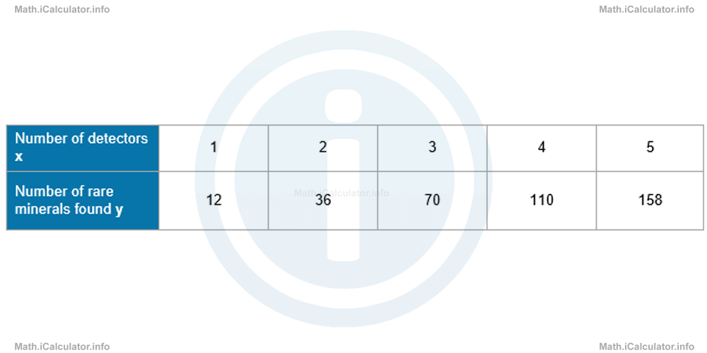
Let's try to identify any relationship of the form y(x) = k · xⁿ. If it exists, the table must transform in such a way that the first row must contain the log x values and the second row the corresponding log y values.

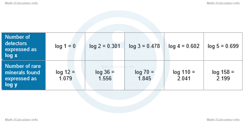
When these points are plotted on a log y vs log x graph yields

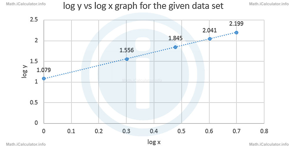
The dashed line shows the trend line (sometimes called the best-fit line), which is straight. This means the original relationship between x and y is of the form

modelled to the above graph through the logarithmic relationship

Now let's calculate the gradient n of the above line, which corresponds to the exponent of the original function. We have

Since all measurements contain their margin of error, we take the rounded value n = 1.6 as the exponent of the original function.

Now, we have to calculate the coefficient k, which in the corresponding logarithmic function is given by log k. It represents the intercept of the line with the log y (vertical) axis on the linear graph shown above. In other words, it shows the initial vertical coordinate when the horizontal coordinate is zero. Given that we have log k = 1.079 which corresponds to the original value of 12 rare minerals when a single detector is used, then k = 12. Hence, the original function that shows the relationship between the number of detectors used and the number of minerals found has the form

As mentioned earlier, knowing the general formula of such a function allows us to make predictions on situations where more elements (here detectors) are involved. In other words, we can make a prediction on how many rare minerals we can find by using more than five detectors.

Example 3

1. Check for any relationship of the form y(x) = k · xⁿ between the quantities involved in the data set collected during an experiment shown in the table below.
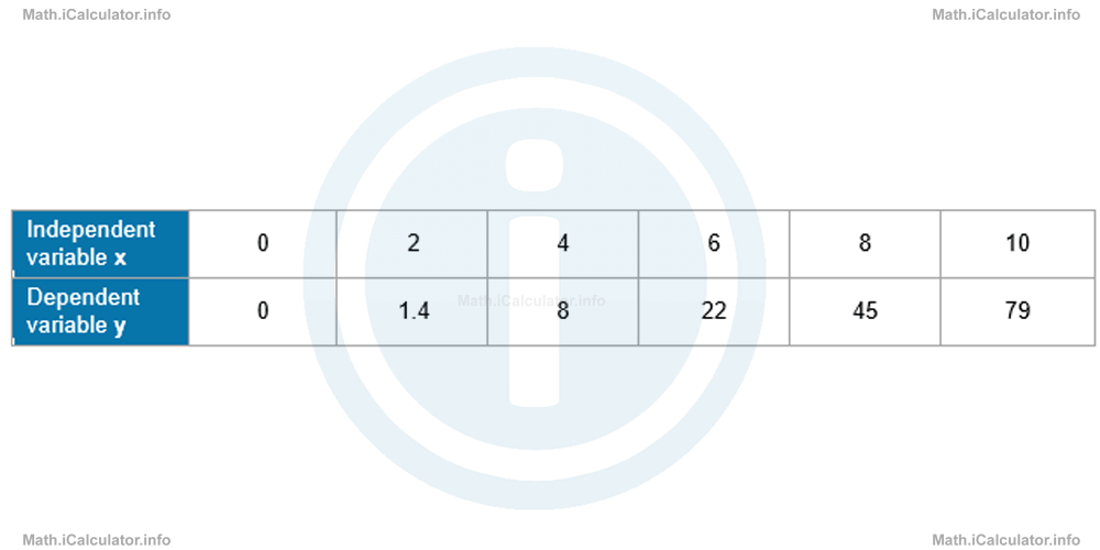
2. If such a relationship exists, find the approximate y-value for x = 20.

Solution 3

1. Let's create a new table where the values of log x and log y are placed instead of the original x- and y-values. 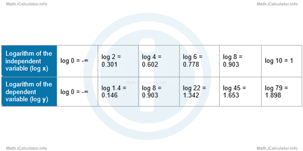(We take log 0 = -∞ because 10^{-∞,/sup> = 0}. Indeed, the graph of a logarithmic function y = log x never touches the y-axis, as the independent variable can only approach zero but never be zero. The more the x-value points towards zero, the more the corresponding y-value points towards minus infinity).
   Now, let's plot the log y vs log x graph for this data set. We can skip the first column, as both values are minus infinity and are not shown in the graph. Thus, we have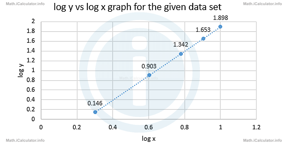 The dashed line shows the trend line (the best-fit line), which is straight. This means the original relationship between x and y is of the form
   y(x) = k ∙ xⁿ
   modelled to the above graph through the logarithmic relationship
   log y = n ∙ log x + log k
   Now let's calculate the gradient n of the above line, which corresponds to the exponent of the original function. (Again, let's skip the minus infinity values). We have
   n = ∆ log y/∆ log x
   = log 79 - log 1.4/log 10 - log 2
   = 1.898 - 0.146/1 - 0.301
   = 1.752/0.699
   = 2.506
   Since all measurements contain their margin of error, we take the rounded value n = 2.5 as the exponent of the original function.
   Now, we have to calculate the value of the coefficient k, as it is not actually shown by the graph. Since the function has the form
   y(x) = k ∙ x².5
   we can substitute in it a pair of coordinates from any point shown by the original table, for example, x = 4 and y = 8. In this way, we obtain
   8 = k ∙ 4^2.5
   8 = k ∙ 32
   k = 32/8
   k = 4
   Therefore, the original function indicated by the first table (and also from the second table and the graph) is
   y(x) = 4 ∙ x^2.5
2. Following this trend, for x = 20 we obtain
   y(x) = 4 ∙ x^2.5
   y(20) = 4 ∙ 20^2.5
   = 4 ∙ 1788.85
   = 7155

2. Functions of the form y(x) = a · b^x

These functions are considered as pure exponential functions as the independent variable is in the exponent. The transformation made in such functions for modelling them is

This form is similar to that of a linear function where log b is the gradient and log a the constant of the line. Therefore, this time we have to plot the log y vs x graph instead of log y vs log x one. This means that only the vertical axis needs to be transformed. For example, if we have the set of the following data that shows the presence of bacteria in a food sample left outside the refrigerator

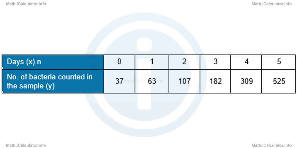
and we want to investigate any exponential relationship in order to find whether they are resistant to environmental conditions (if there is any sustainable exponential relationship, this means the bacteria are resistant and keep growing in number according to a certain proliferation rate), then we follow the procedure described earlier in theory.

Thus, it is obvious that if there is a relationship between the variables similar to those explained earlier then the value of the coefficient b of this function is 37 as this is the original number of bacteria in the sample (this is because a⁰ = 1). Hence, the possible function has the general form.

Now, let's try to confirm this possible exponential relationship by modelling the curve by using logarithms. This means we have to consider log y instead of y in the above table. In this way, we obtain the following new table

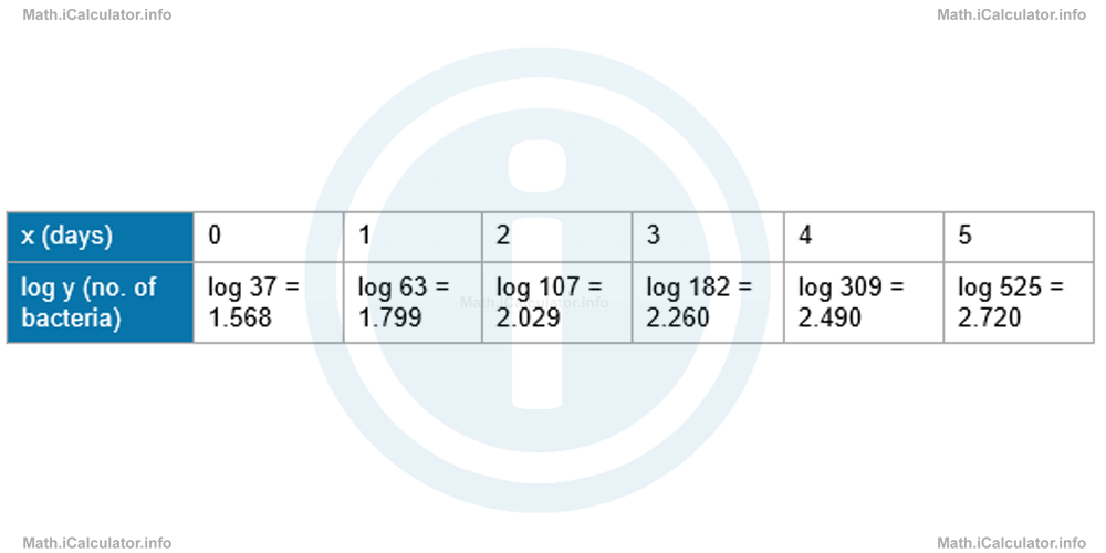
When plotting these values on a log y vs x graph yields

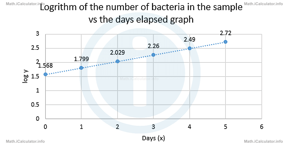
The trend line indicates a linear relationship. Therefore, we have a function of the form

The procedure used to find the missing coefficients is as follows:

Step 1: First, we determine the constant log a. This represents the value of log y for x = 0. In other words, it represents the initial vertical coordinate of the line, i.e. log a = log (0). From the second table, we know that for x = 0, log y = 1.568. Therefore, log a = 1.568. Hence, the above function becomes

Step 2: Then, we calculate the gradient log b of the line using the relation

Taking the initial and the first coordinates yields

Step 3: Then, we calculate the value of b through the relation

In this way, we obtain the value of b in the original function

Hence, the original relationship between the number of days elapsed and the number of bacteria in the sample is

Example 4

The mass of an avalanche in kilograms as a function of the sliding distance from the top of a mountain expressed in decametres (dam), where 1 dam = 10 m, is shown in the table below.

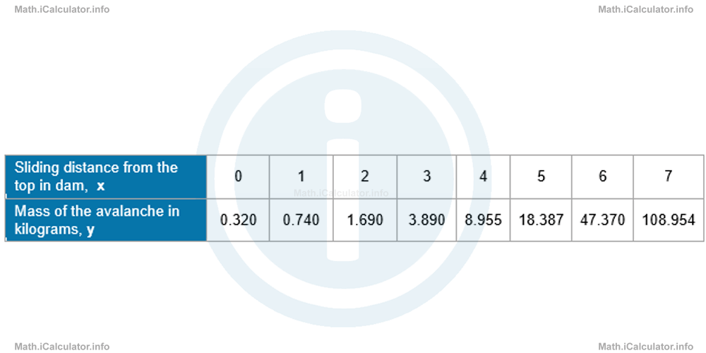
Find:

1. The mass of avalanche v's sliding distance function determined by the above data.
2. The mass of the avalanche when the slow slides down the mountain to 200 m below the original position.

Solution 4

1. The mass of the avalanche increases more than twice for each decametre when falling down the top of the mountain. Therefore, there must be some sort of exponential function involved. However, to be confident of this hypothesis, we find the logarithms of all y-values representing the mass and see whether there is any linear relationship between the new values obtained and those of the distance. In this way, we obtain the following table. 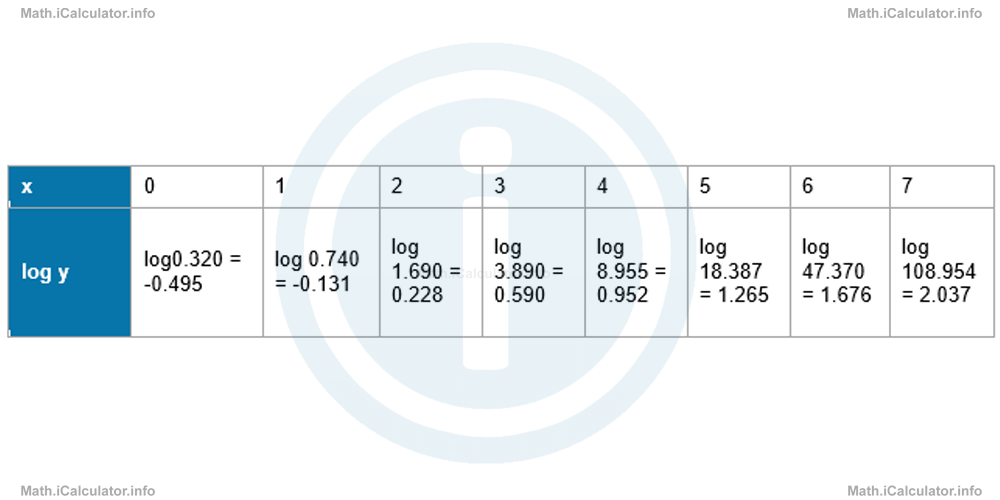When plotting the above data in the log y v's x graph yields 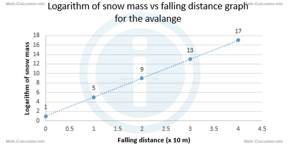Therefore, it is already certain that the original function has the form
   y(x) = a ∙ b^x
   Now, let's find the coefficient a. From the original table you can see that for x = 0, y = 0.320. Since b^x = b⁰ = 1, then a = y(0) = 0.320. As for the base b, we can substitute the coordinates of any point in the original graph. For example, for x = 1 and y = 0.740 we obtain
   y = a ∙ b^x
   0.740 = 0.320 ∙ b¹
   b = 0.740/0.320
   b = 2.3
   Hence, the snow mass of the avalanche increases for every falling decametre according to the exponential function
   y(x) = 0.320 ∙ 2.3^x
2. If the avalanche slides down for 200 m or 20 dam (x = 20), its mass becomes
   y(20) = 0.320 ∙ 2.3²0
   = 5,491,699 kg
   This is a very large amount of snow, although in reality a part of the snow collected in the avalanche detaches from it on the way. More importantly, the remaining part is large enough to cause harm to property and people.

How to understand a-priori whether a function is of the form y(x) = k · xⁿ or y(x) = b · a^x?

This is not merely a question of experience (although experience plays an important role in guiding your intuition towards the right path) but of the reasoning as well. You must take a look at the first two or three columns of the table and see whether there is any kind of geometric progression in the values. In this case, the function most probably has the form y(x) = b · a^x. If you are not able to identify such a relationship that resembles a geometric sequence but the values look more like forming an arithmetic one (albeit not exactly), then try the first option, i.e. y(x) = k · xⁿ.

More Modelling Curves using Logarithms Lessons and Learning Resources

Logarithms Learning Material

Tutorial ID	Math Tutorial Title	Tutorial	Video Tutorial	Revision Notes	Revision Questions
13.3	Modelling Curves using Logarithms
Lesson ID	Math Lesson Title			Lesson	Video Lesson
13.3.1	A Brief Introduction to Functions
13.3.2	Exponential Function Graphs
13.3.3	Finding the Formula of an Unknown Exponential Function
13.3.4	Logarithmic Function Graphs
13.3.5	Modelling Curves Using Logarithms

Whats next?

Enjoy the "Modelling Curves Using Logarithms" math lesson? People who liked the "Modelling Curves using Logarithms lesson found the following resources useful:

1. Modelling Curves Feedback. Helps other - Leave a rating for this modelling curves (see below)
2. Logarithms Math tutorial: Modelling Curves using Logarithms. Read the Modelling Curves using Logarithms math tutorial and build your math knowledge of Logarithms
3. Logarithms Video tutorial: Modelling Curves using Logarithms. Watch or listen to the Modelling Curves using Logarithms video tutorial, a useful way to help you revise when travelling to and from school/college
4. Logarithms Revision Notes: Modelling Curves using Logarithms. Print the notes so you can revise the key points covered in the math tutorial for Modelling Curves using Logarithms
5. Logarithms Practice Questions: Modelling Curves using Logarithms. Test and improve your knowledge of Modelling Curves using Logarithms with example questins and answers
6. Check your calculations for Logarithms questions with our excellent Logarithms calculators which contain full equations and calculations clearly displayed line by line. See the Logarithms Calculators by iCalculator™ below.
7. Continuing learning logarithms - read our next math tutorial: Natural Logarithm Function and Its Graph

Help others Learning Math just like you

Please provide a rating, it takes seconds and helps us to keep this resource free for all to use

We hope you found this Math tutorial "Modelling Curves using Logarithms" useful. If you did it would be great if you could spare the time to rate this math tutorial (simply click on the number of stars that match your assessment of this math learning aide) and/or share on social media, this helps us identify popular tutorials and calculators and expand our free learning resources to support our users around the world have free access to expand their knowledge of math and other disciplines.

Logarithms Calculators by iCalculator™