Math Lesson 15.5.7 - Exponential Graphs with Negative Base

Please provide a rating, it takes seconds and helps us to keep this resource free for all to use

Welcome to our Math lesson on Exponential Graphs with Negative Base, this is the seventh lesson of our suite of math lessons covering the topic of Exponential Graphs, you can find links to the other lessons within this tutorial and access additional Math learning resources below this lesson.

Exponential Graphs with Negative Base

Now, let's see what happens to the graph if the base of an exponential function is negative. Again, let's compare it with the parent function with the same but positive base. For simplicity, we take again y(x) = 2x as a parent function, as it gives smaller numbers. We will compare its graph with that of y(x) = -2x to see how they differ. From a quick look, it is evident that all y-values of the new function will be the same as those of the parent function but with negative sign. This means the graph of y(x) = -2x is obtained by flipping vertically the graph of y(x) = 2x. Hence, we conclude that any negative sign preceding the base inverts an exponential graph down, as occurs with all the other types of graphs as well. Look at the figure below.

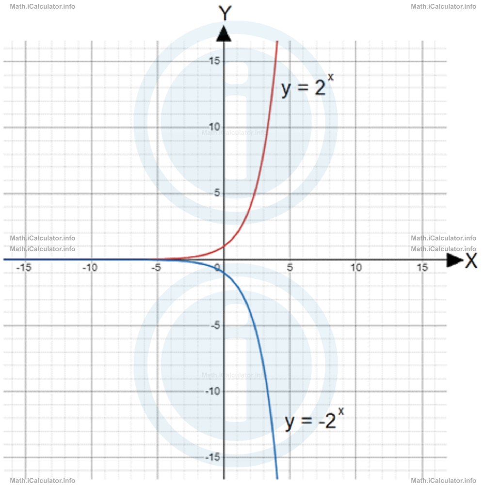
The asymptote (here it is y = 0) helps a lot in this regard, as you can plot a symmetrical figure where the asymptote of the corresponding function but with a positive base, acts as a symmetry axis for the graphs.

Example 6

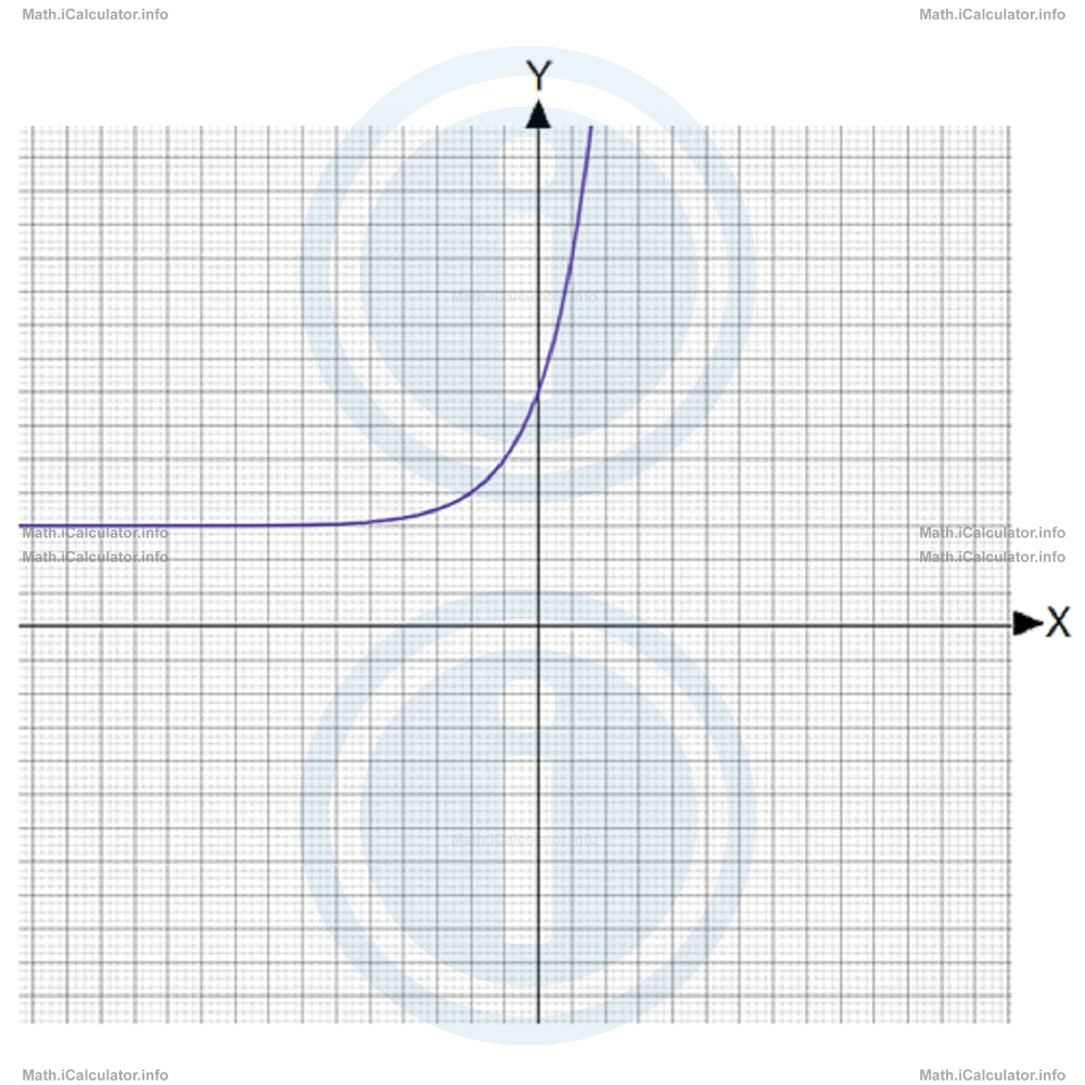
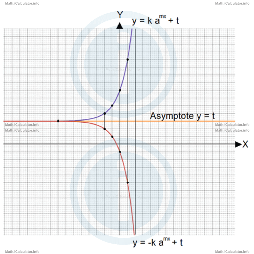
Plot the graph of the exponential function y = -k · ax + t with the help of the graph of y = k · ax + t shown in the figure. The units are unknown, i.e. it is not known how many units each square represents.

Solution 6

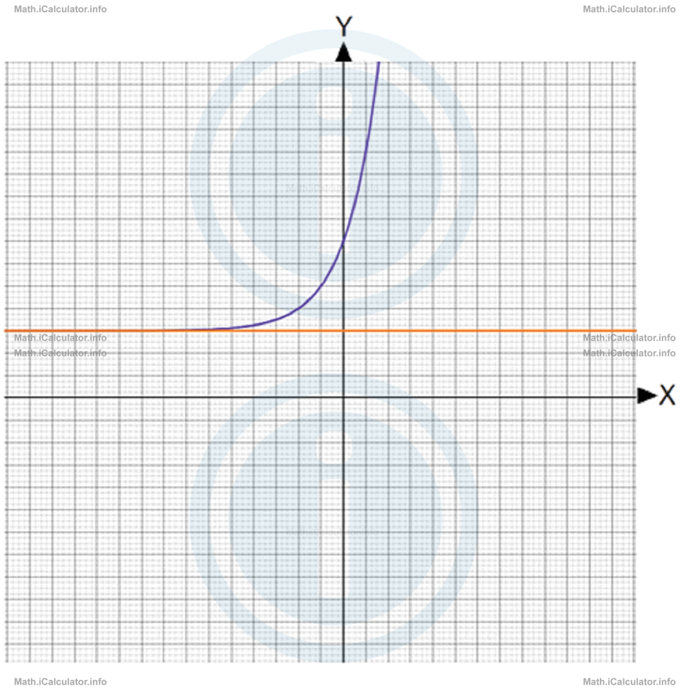
Since no units are given, it is impossible to rely on finding the formula of the function. The only way to plot the graph of the required function is to apply the symmetry with respect to a horizontal line, which here corresponds to the asymptote of the function. You can easily see that the asymptote lies three big squares above the horizontal axis, as shown below.

The next step requires identifying some points in the original graph and inserting some corresponding points below the asymptote for each of them, at the same distance from the asymptote, as shown below.

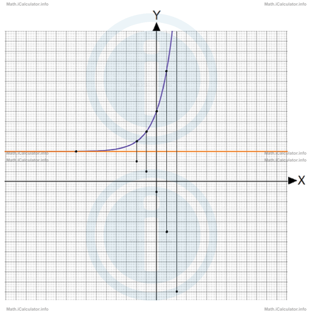
The vertical bars are shown with the purpose to clarify the procedure, i.e. they help to keep the direction and distance from the asymptote.

Now, we connect smoothly the points below the asymptote to plot the required graph, as shown below.

We took into consideration only five points, as this was just for illustration purpose. The more points you include in the graph, the more accurate it becomes.

You have reached the end of Math lesson 15.5.7 Exponential Graphs with Negative Base. There are 8 lessons in this physics tutorial covering Exponential Graphs, you can access all the lessons from this tutorial below.

More Exponential Graphs Lessons and Learning Resources

Whats next?

Enjoy the "Exponential Graphs with Negative Base" math lesson? People who liked the "Exponential Graphs lesson found the following resources useful:

1. Negative Base Feedback. Helps other - Leave a rating for this negative base (see below)
2. Types of Graphs Math tutorial: Exponential Graphs. Read the Exponential Graphs math tutorial and build your math knowledge of Types of Graphs
3. Types of Graphs Revision Notes: Exponential Graphs. Print the notes so you can revise the key points covered in the math tutorial for Exponential Graphs
4. Types of Graphs Practice Questions: Exponential Graphs. Test and improve your knowledge of Exponential Graphs with example questins and answers
5. Check your calculations for Types of Graphs questions with our excellent Types of Graphs calculators which contain full equations and calculations clearly displayed line by line. See the Types of Graphs Calculators by iCalculator™ below.
6. Continuing learning types of graphs - read our next math tutorial: Circle Graphs

Help others Learning Math just like you

Please provide a rating, it takes seconds and helps us to keep this resource free for all to use

We hope you found this Math tutorial "Exponential Graphs" useful. If you did it would be great if you could spare the time to rate this math tutorial (simply click on the number of stars that match your assessment of this math learning aide) and/or share on social media, this helps us identify popular tutorials and calculators and expand our free learning resources to support our users around the world have free access to expand their knowledge of math and other disciplines.

Types of Graphs Calculators by iCalculator™