Menu
Math Lesson 15.8.4 - Calculating the Gradient of a Curve: Gradient of a cubic function
Please provide a rating, it takes seconds and helps us to keep this resource free for all to use
Welcome to our Math lesson on Calculating the Gradient of a Curve: Gradient of a cubic function, this is the fourth lesson of our suite of math lessons covering the topic of Gradient of Curves, you can find links to the other lessons within this tutorial and access additional Math learning resources below this lesson.
Calculating the Gradient of a Curve: Gradient of a cubic function
In the previous lesson we explained how to find the gradient's formula for a quadratic function, it is much easier to understand the method used to find the gradient's formula of a cubic function because the approach is identical. Thus, first we deal with the parent cubic function f(x) = x3 and use the known steps to find the general formula of its gradient. As usual first we take a sample point with x-coordinate x0 and consider a small change Δx in the x-coordinate. As a result, the y-coordinate will change by Δy as well. We have
f(x0 + ∆x) = (x0 + ∆x)3
= x30 + 3x20 ∙ ∆x + 3x0 ∙ ∆x20 + ∆x30
The next step involves finding the difference between f(x0 + Δx) and f(x0). We have
= x30 + 3x20 ∙ ∆x + 3x0 ∙ ∆x20 + ∆x30 - x30
= 3x20 ∙ ∆x + 3x0 ∙ ∆x20 + ∆x30
The last expression shows the change in the y-coordinate (Δy) of the function for the interval chosen. Dividing it by the change Δx in the corresponding x-coordinate for the same interval, gives the gradient k of the parent cubic function, i.e.
= f(x0 + ∆x) - f(x0 )/∆x
= 3x20 ∙ ∆x + 3x0 ∙ ∆x20 + ∆x30/∆x
= ∆x(3x20 + 3x0 ∙ ∆x0 + ∆x30)/∆x
= 3x20 + 3x0 ∙ ∆x0 + ∆x30
Again, neglecting the terms containing Δx because very small (as we did in the quadratic function) yields
Generalizing for any x, yields the general formula of the gradient of parent cubic function
Remark! You may be confused about the fact that the gradient's equation of the parent cubic function is quadratic. This may lead to the wrong conclusion that the tangent to the cubic graph at a given point is not linear but a parabola. However, the concept of the gradient of a function is not the same as that of the tangent to a line. In fact, the gradient shows the linear coefficient of the tangent line to the given point, not the equation of the tangent itself. More precisely, the gradient shows only the coefficient k preceding the variable x in the equation of tangent y = kx + t. Let's clarify this point through an example.
Example 4
- Calculate the gradient of the parent cubic function f(x) = x3 at points A and B with horizontal coordinates xA = -2 and xB = 1. Use the substitution of surrounding values to the given to find the gradient in each case.
- Check the results obtained in (a) by using the specific formula for the gradient of the parent cubic function.
- Find the equation of the tangent lines to the graph at points A and B.
- Plot the graph of the function including the tangent lines at points A and B.
Solution 4
- As usual, we consider two points aside the given point, very close to it. Thus, for point A we choose x1 = -2.1 and x2 = -1.9. In this way, we have for the corresponding y-values: y1 = x31and
= (-2.1)3
= -9.261y2 = x32Therefore, the gradient at point A is
= (-1.9)3
= -6.859kA = y2 - y1/x2 - x1Note the small fluctuation from the true value (12) which occurs because of the error when taking the small arc as a straight line.
= -6.859 - (-9.261)/(-1.9) - (-2.1)
= -6.859 + 9.261/-1.9 + 2.1
= 2.402/0.2
= 12.01
The same procedure is followed when calculating the gradient kB at point B as well. Thus, the y-values for for x1 = 0.9 and x2 = 1.1 arey1 = x31and
= (0.9)3
= 0.729y2 = x32Therefore, the gradient k at point B is
= (1.1)3
= 1.331kB = y2 - y1/x2 - x1Again, we round this value to kB = 3, as the small fluctuations are because the error when taking the small arc as a straight line.
= 1.331 - 0.729/1.1 - 0.9
= 0.602/0.2
= 3.01 - Given that the formula for calculating the gradient of f(x) = x3 is k = 3x2, we obtain for the gradients in the given points: kA = 3 ∙ x2Aand
= 3 ∙ (-2)2
= 3 ∙ 4
= 12kB = 3 ∙ x2BThese results are the same as those obtained in (a) but in a much shorter way.
= 3 ∙ 12
= 3 ∙ 1
= 3 - The equation of tangents at points A and B are y = kA ∙ x + t1and
= 12x + t1y = kB ∙ x + t2where t1 and t2 are the constants of each of the tangents at the given points. Let's find the y-coordinates of these points so that after substituting the two coordinates of each point in the corresponding tangent's formulas we are able to find the two constants t1 and t2.
= 3x + t2
Thus, for the point A (x = -2) we haveyA = x3Aand
= (-2)3
= -8yB = x3BTherefore, the coordinates of points A and B are A(-2, -8) and B(1, 1). Substituting these points in the tangent's formulas yields
= 13
= 1yA = kA ∙ xA + t1and
-8 = 12 ∙ (-2) + t1
-8 = -24 + t1
t1 = -8 + 24
t1 = 16yB = kB ∙ xB + t2Therefore, the tangent lines with the graph of the parent cubic function f(x) = x3 at A(-2, 8) and B(1, 1) are
1 = 3 ∙ 1 + t2
1 = 3 + t2
t2 = 1 - 3
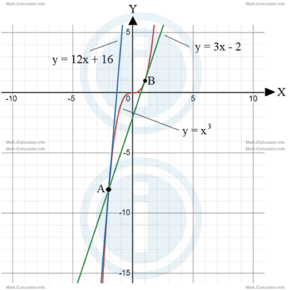
t2 = -2y = 12x + 16andy = 3x - 2respectively. - The graph of the function f(x) = x3 as well as the tangents at points A and B are shown in the graph below.
 Now, let's see what happens when dealing with cubic functions of the general form f(x) = ax3 + bx2 + cd + dSince the right side of this function represents a polynomial, the gradients are calculated separately, i.e. each term has its own gradient. We have four gradients to calculate; one for each term. Thus, we haveTerm 1 = ax3 ⟶ k1 = 3ax2Therefore, the gradient of the general cubic function is
Term 2 = bx2 ⟶ k2 = 2bx
Term 3 = cx ⟶ k3 = c
Term 4 = d ⟶ k4 = 0k = k1 + k2 + k3 + k4For example, the gradient of f(x) = 2x3 + 4x2 - x + 5 (a = 2, b = 4, c = -1 and d = 5) is
= 3ax2 + 2bx + c + 0
= 3ax2 + 2bx + ck = 3ax2 + 2bx + cDespite the gradient of this function has only this formula, the value of gradient varies depending on the points chosen. Thus, if we choose for example the gradient at a point with x-coordinate x = 0, the gradient is
= 3 ∙ 2 ∙ x2 + 2 ∙ 4 ∙ x + (-1)
= 6x2 + 8x - 1k = 6x2 + 8x - 1On the other hand, if we choose another point with x-coordinate x = 2, the gradient is
= 6 ∙ 02 + 8 ∙ 0 - 1
= -1k = 6x2 + 8x - 1Again, these gradients show only the coefficient preceding the variable x in the equation of tangent lines at the given points, not the equations themselves. Let's see an example.
= 6 ∙ 22 + 8 ∙ 2 - 1
= 24 + 16 - 1
= 39
Example 5
- Find the gradients of f(x) = x3 - 2x2 - 5x + 3 at the points A and B with horizontal coordinates xA = 0 and xB = 3 using the gradient's equation for this function explained in theory.
- Check the correctness of the result obtained through the long way, i.e. by using the two-surrounding-points method.
- Find the equation of tangents to the function at the given points A and B.
- Plot the graph of the function including the tangent lines at points A and B.
Solution 5
- This is a cubic function of the type f(x) = ax3 + bx2 + cx + d where in the specific case we have a = 1, b = -2, c = -5 and d = 3.
From the general gradient's formula for this type of function k = 3ax2 + 2bc + c, we obtain for the gradient's formula of this specific functionk = 3ax2 + 2bx + cThus, the values of gradient at points A and B (where xA = 0 and xB = 3) are
= 3 ∙ 1 ∙ x2 + 2 ∙ (-2) ∙ x + (-5)
= 3x2 - 4x - 5kA = 3x2A - 4xA-5and
= 3 ∙ 02 - 4 ∙ 0 - 5
= 0 - 0 - 5
= -5kB = 3x2B - 4xB - 5
= 3 ∙ 32 - 4 ∙ 3 - 5
= 27 - 12 - 5
= 10 - Now, let's check whether the values found above are correct or not. For this, we have to use the long method, which involves the calculation of gradient by its definition, i.e. by the formula k = ∆y/∆x = y2 - y1/x2 - x1where (x1, y1) are the coordinates of a point before A very close to it, while (x2, y2) are the coordinates of another point after A, very close to it. The same procedure is carried out for point B as well.
As usual, we choose two points that are 0.1 units away from the given point in which we want to calculate the gradient, in both of its sides. Thus, for point A we choose x1 = -0.1 and x2 = 0.1, while for point B we choose x1 = 2.9 and x2 = 3.1. The corresponding y-value for these four points are as following:
Around point A we havey1 = x31 - 2x21 - 5x1 + 3and
= (-0.1)3 - 2 ∙ (-0.1)2 - 5 ∙ (-0.1) + 3
= -0.001 - 2 ∙ 0.01 - 5 ∙ (-0.1) + 3
= -0.001 - 0.02 + 0.5 + 3
= 3.479y2 = x32 - 2x22 - 5x2 + 3Thus, the gradient at point A is
= (0.1)3 - 2 ∙ (0.1)2 - 5 ∙ (0.1) + 3
= 0.001 - 2 ∙ 0.01 - 5 ∙ (0.1) + 3
= 0.001 - 0.02 - 0.5 + 3
= 2.481kA = ∆yA/∆xAWe write this result as kA = -5. It is the same number obtained at (a) for the gradient at point A. Likewise, for the part of the graph around point B we have
= y2 - y1/x2 - x1
= 2.481 - 3.479/0.1 - (-0.1)
= -0.998/0.2
= -4.99y1 = x31 - 2x21 - 5x1 + 3and
= (2.9)3-2 ∙ (2.9)2-5 ∙ (2.9) + 3
= 24.389 - 2 ∙ 8.41-5 ∙ 2.9 + 3
= 24.389 - 16.82 - 14.5 + 3
= -3.931y2 = x32 - 2x22 - 5x2 + 3Thus, the gradient at point B is
= (3.1)3 - 2 ∙ (3.1)2 - 5 ∙ (3.1) + 3
= 29.791 - 2 ∙ 9.61 - 5 ∙ (3.1) + 3
= 29.791 - 19.22 - 15.5 + 3
= -1.929kB = ∆yB/∆xBWe write this result as kB = 10. It is the same number obtained at (a) for the gradient at point B.
= y2 - y1/x2 - x1
= -1.929 - (-3.931)/3.1 - 2.9
= -1.929 + 3.931/3.1 - 2.9
= 2.002/0.2
= 10.01 - The general equation of the tangent in each point of the graph is y = kx + t, where k is the gradient. Thus, for point A we have yA = kA ∙ xA + t1and for point B we haveyB = kB ∙ xB + t2where t1 and t2 are the tangent line constants at points A and B.
From the original function we obtain for yA and yByA = x3A - 2x2A - 5xA + 3and
= 03-2 ∙ 02 - 5 ∙ 0 + 3
= 0-2 ∙ 0 - 5 ∙ 0 + 3
= 0 - 0 - 0 + 3
= 3yB = x3B - 2x2B - 5xB + 3Therefore, for the gradient at point A we have
= 33-2 ∙ 32 - 5 ∙ 3 + 3
= 27 - 2 ∙ 9 - 5 ∙ 3 + 3
= 27 - 18 - 15 + 3
= -3yA = kA ∙ xA + t1and for the gradient at point B we have
3 = -5 ∙ 0 + t1
t1 = 3yB = kB ∙ xB + t2Therefore the equations of the two gradients at points A and B are
-3 = 10 ∙ 3 + t2
-3 = 30 + t2
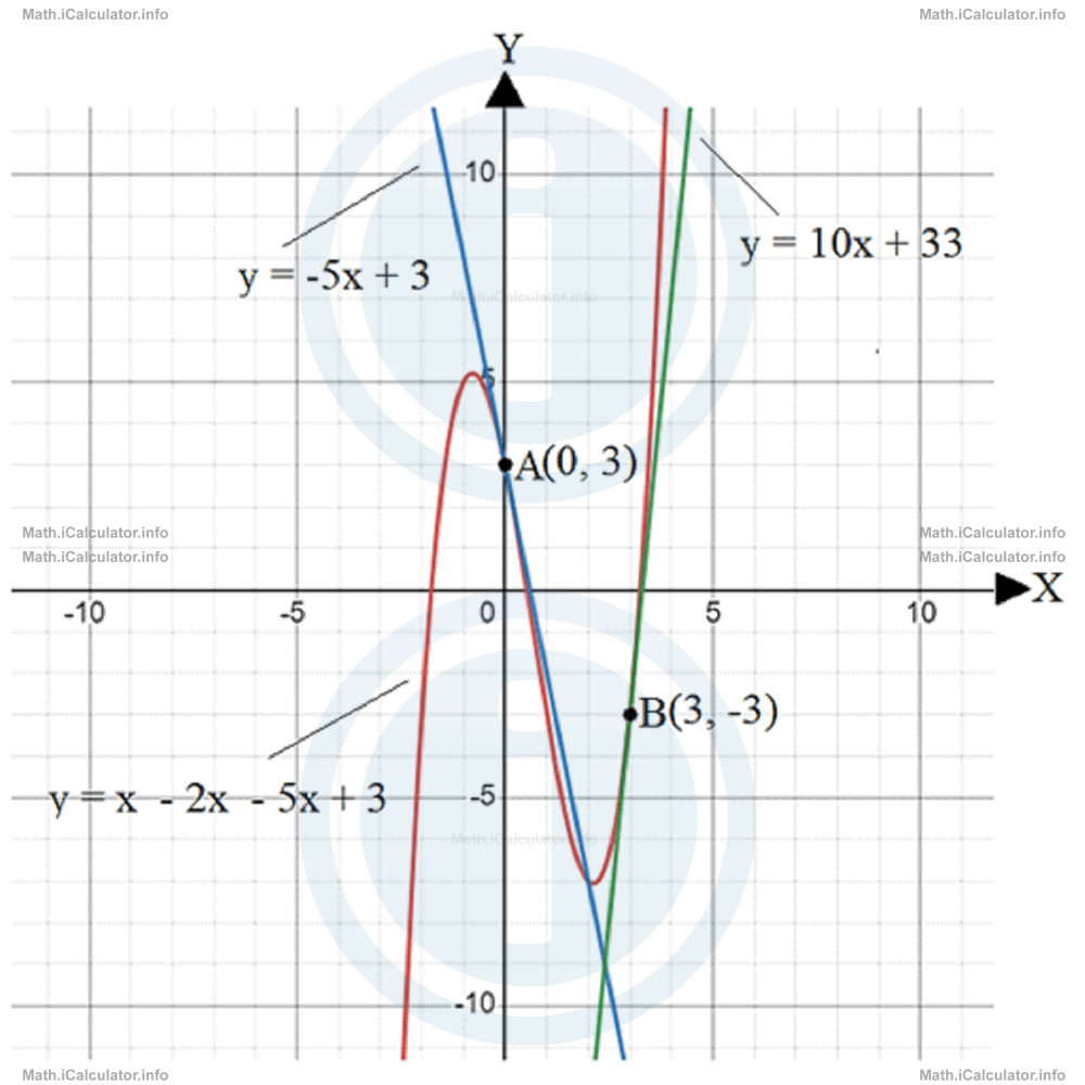
t2 = -33y = -5x + 3andy = 10x - 33 - The figure below shows the graph of the cubic function f(x) = x3 - 2x2 - 5x + 3 as well as the tangent lines at points A(0, 3) and B(3, -3).
You have reached the end of Math lesson 15.8.4 Calculating the Gradient of a Curve: Gradient of a cubic function. There are 4 lessons in this physics tutorial covering Gradient of Curves, you can access all the lessons from this tutorial below.
More Gradient of Curves Lessons and Learning Resources
Whats next?
Enjoy the "Calculating the Gradient of a Curve: Gradient of a cubic function" math lesson? People who liked the "Gradient of Curves lesson found the following resources useful:
- Cubic Function Feedback. Helps other - Leave a rating for this cubic function (see below)
- Types of Graphs Math tutorial: Gradient of Curves. Read the Gradient of Curves math tutorial and build your math knowledge of Types of Graphs
- Types of Graphs Revision Notes: Gradient of Curves. Print the notes so you can revise the key points covered in the math tutorial for Gradient of Curves
- Types of Graphs Practice Questions: Gradient of Curves. Test and improve your knowledge of Gradient of Curves with example questins and answers
- Check your calculations for Types of Graphs questions with our excellent Types of Graphs calculators which contain full equations and calculations clearly displayed line by line. See the Types of Graphs Calculators by iCalculator™ below.
- Continuing learning types of graphs - read our next math tutorial: Quadratic Graphs Part One
Help others Learning Math just like you
Please provide a rating, it takes seconds and helps us to keep this resource free for all to use
We hope you found this Math tutorial "Gradient of Curves" useful. If you did it would be great if you could spare the time to rate this math tutorial (simply click on the number of stars that match your assessment of this math learning aide) and/or share on social media, this helps us identify popular tutorials and calculators and expand our free learning resources to support our users around the world have free access to expand their knowledge of math and other disciplines.