Math Lesson 16.3.3 - Cubic Functions

Please provide a rating, it takes seconds and helps us to keep this resource free for all to use

Welcome to our Math lesson on Cubic Functions, this is the third lesson of our suite of math lessons covering the topic of Basic Functions, you can find links to the other lessons within this tutorial and access additional Math learning resources below this lesson.

Cubic Functions

Cubic functions have a general form of

where a, b and c are coefficients while d is a constant.

If factorization is possible, we can write the cubic function as a product of a linear and a quadratic function. For example, we can transform the cubic function

in the following way:

This helps identify the zeroes of the cubic function (which is a polynomial function) by solving the equation f(x) = 0. In our example, we have to solve the equation

to find the roots (zeroes) of the original function, which gives us the x-intercepts of the corresponding graph. The first expression becomes zero for x = 2. As for the second expression, we have to solve the quadratic equation

where a = 1, b = -3 and c = 1.

The discriminant Δ of this equation is

Thus, since the discriminant is positive, the above quadratic equation has two distinct roots,

and

Therefore, the function f(x) intercepts the horizontal axis at three points: (0.382, 0), (2.618, 0) and (5, 0).

Another thing we have already dealt with that regards cubic functions is the gradient. In tutorial 15.8, we explained that the gradient m of the cubic function

is

Obviously, the gradient is different for different values of x. Since the gradient m gives the steepness of the tangent line to the graph at the given point, it is clear that there is an infinity of possible lines that can be tangent to the graph at different points. The general equation of all such tangents is

where n is a constant.

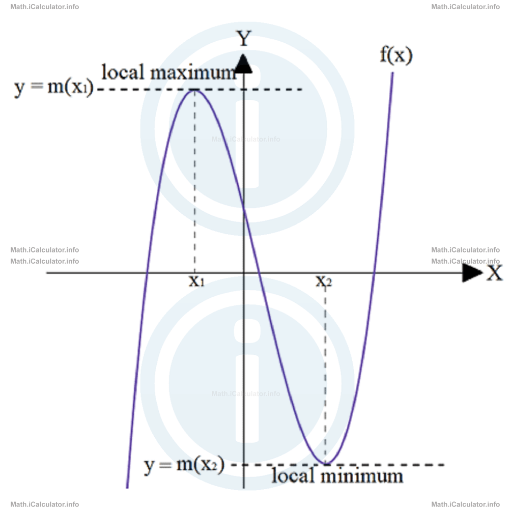
Another thing we can do with the gradient is to find any local minimum or maximum of the function. Thus, a tangent line y = m(x) must act as a kind of "floor" at the local minimum point of a graph or as a "roof" at the local maximum point, both of these tangent lines must be horizontal. Hence, the gradient must be zero at the local minimum or at the local maximum point of a function. This is true for all functions, including cubic ones.

Remark! We say "local" minimum or maximum because the graph may extend to infinity but we are interested in the wiggle formed when the graph line changes direction.

As for the domain and range of cubic functions, they are unlimited unless a restriction is explicitly given in the clues.

Last, we can find the y-intercept by substituting x = 0 in the original function, i.e. by finding f(0).

Example 3

For the cubic function

find:

1. The gradient at x = 2
2. The local maximum and/or minimum of this function
3. The x-intercepts
4. The y-intercept
5. Plot the graph including all relevant points used for this purpose

Solution 3

1. First, we have to find the formula of the gradient m. In this function, we have a = 1, b = 6, c = -7 and d = 6. Given that the general formula of the gradient of a cubic function is
   m = 3ax² + 2bx + c
   we obtain for this specific gradient
   m = 3 · 1 · x² + 2 · 6 · x + (-7)
   m = 3x² + 12x - 7
   Therefore, for x = 2, the gradient is
   m(2) = 3 · 2² + 12 · 2 - 7
   = 3·4 + 12 · 2 - 7
   = 12 + 24 - 7
   = 29
2. The local maximum and minimum of a function are found by solving the equation m(x) = 0, where m(x) is the gradient(s) at the point(s) x. Thus, we have to solve the equation
   3x² + 12x - 7 = 0
   In this quadratic equation, we have a = 3, b = 12 and c = -4. The discriminant Δ is
   ∆ = b² - 4ac
   = 12²-4 ∙ 3 ∙ (-7)
   = 144 + 84
   = 228
   Since the discriminant is positive, this equation has two roots:
   x₁ = -b - √∆/2a
   = -12 - √228/2 ∙ 3
   = -12 - 15.1/6
   = -4.52
   and
   x₂ = -b + √∆/2a
   = -12 + √228/2 ∙ 3
   = -12 + 15.1/6
   = 0.52
   The corresponding y-values represent the local minimum and maximum of this function. Thus, for x = -4.52 we have
   f(-4.52) = (-4.52)³ + 6 ∙ (-4.52)² - 7 ∙ (-4.52) - 6
   = -92.3 + 122.6 + 31.6 - 6
   = 55.9
   ≈ 56
   and for x = 0.52 we have
   f(0.52) = (0.52)³ + 6 ∙ (0.52)² - 7 ∙ (0.52) - 6
   = 0.14 + 1.62 - 3.64 - 6
   = -7.9
   ≈ -8
   Therefore, the local minimum of the function is y_min = -8, while the local maximum is y_max = 56.
3. The x-intercepts are found by solving the cubic equation f(x) = 0. We are not able to identify any useful factorization, so we solve this part of the exercise using the iterative methods in the sense that since x = 0.52 (where f(0.52) = -8) is a local minimum and x = -4.52 (where f(-4.52) = 56) is a local maximum of the function, there must be an x-intercept between these two values. Thus, for x = -2, we have
   f(-2) = (-2)³ + 6 ∙ (-2)² - 7 ∙ (-2) - 6
   = -8 + 6 ∙ 4 - 7 ∙ (-2)
   = -8 + 24 + 14
   = 30
   Thus, one of the roots (x-intercepts) is between x = 0.52 and x = -2 because the corresponding images f(x) have opposite sign (recall the tutorial 9.4).
   Again, we can take x = -1 and see what is the corresponding f(x). Thus,
   f(-1) = (-1)³ + 6 ∙ (-1)² - 7 ∙ (-1) - 6
   = -1 + 6 ∙ 1 - 7 ∙ (-1)
   = -1 + 6 + 7
   = 12
   Therefore, the root will be between x = 0.52 and x = -1. Again, for x = 0, we have
   f(0) = (0)³ + 6 ∙ (0)²-7 ∙ (0) - 6
   = -6
   This means the root is between 0 and -1. Continuing this way, we find the value x = -0.6 as one of the roots.
   It is known from previous chapters that a cubic equation may have three roots at maximum. Therefore, we must check for two other possible roots, which act as x-intercepts for the graph. These roots must be such that the x-coordinate of the local minimum or maximum be between the new potential root and that identified earlier. In other words, if the function has three zeroes, one of the zeroes must be on the left of x = -4.52 and the other on the right of x = 0.52.
   Using again the iterative method, yields x = -6.9 and x = 1.5 when written at one decimal place. Therefore, we have three x-intercepts of the f(x) graph: (-6.9, 0), (-0.6, 0) and (1.5, 0).
4. Since f(x) is a function, there is a single y-intercept of the graph obtained for x = 0. We found earlier that f(0) = -6, so the y-intercept is at (0, -6).
5. Before showing the graph with a solid line, we will show only the points and the auxiliary lines found so far to give a better idea about their importance in plotting the graph.

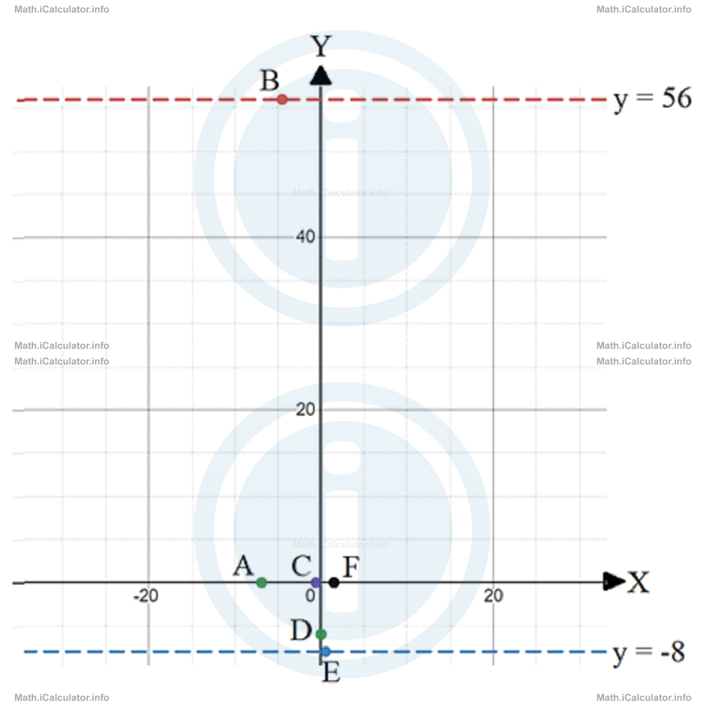
The two dashed lines are the tangents at the points B and E where the gradient is zero. These points correspond to the local maximum and minimum of the function.

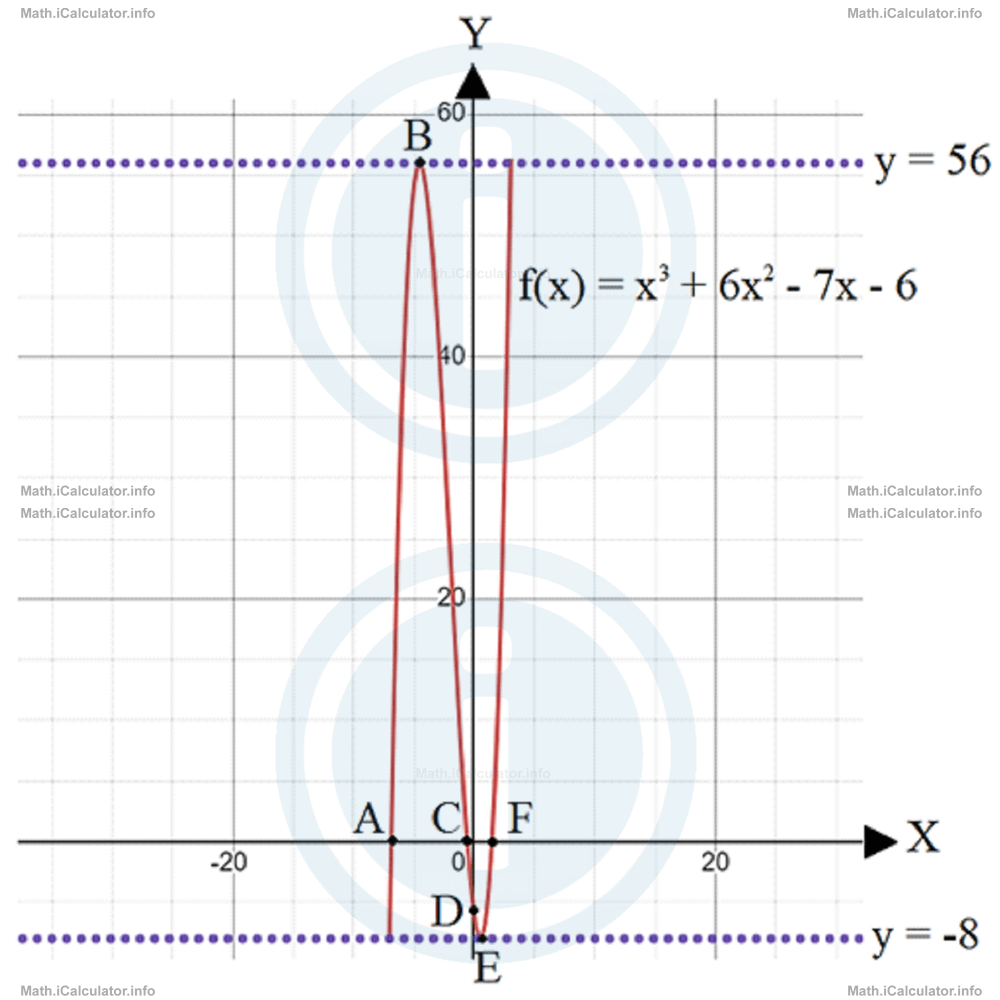
The graph line comes from the infinity from the bottom left side; it goes up through point A(-6.9, 0); again up to the local maximum B(-4.52, 56); then, the graph goes down to the horizontal axis at point C(-0.6, 0); again down to the y-intercept D(0, -6); then to the local minimum E(0.52, -8); then through point F(1.5, 0) and up to the infinity. After joining the above points smoothly, we obtain the following graph.

You have reached the end of Math lesson 16.3.3 Cubic Functions. There are 8 lessons in this physics tutorial covering Basic Functions, you can access all the lessons from this tutorial below.

More Basic Functions Lessons and Learning Resources

Whats next?

Enjoy the "Cubic Functions" math lesson? People who liked the "Basic Functions lesson found the following resources useful:

1. Cubic Feedback. Helps other - Leave a rating for this cubic (see below)
2. Functions Math tutorial: Basic Functions. Read the Basic Functions math tutorial and build your math knowledge of Functions
3. Functions Revision Notes: Basic Functions. Print the notes so you can revise the key points covered in the math tutorial for Basic Functions
4. Functions Practice Questions: Basic Functions. Test and improve your knowledge of Basic Functions with example questins and answers
5. Check your calculations for Functions questions with our excellent Functions calculators which contain full equations and calculations clearly displayed line by line. See the Functions Calculators by iCalculator™ below.
6. Continuing learning functions - read our next math tutorial: Composite Functions

Help others Learning Math just like you

Please provide a rating, it takes seconds and helps us to keep this resource free for all to use

We hope you found this Math tutorial "Basic Functions" useful. If you did it would be great if you could spare the time to rate this math tutorial (simply click on the number of stars that match your assessment of this math learning aide) and/or share on social media, this helps us identify popular tutorials and calculators and expand our free learning resources to support our users around the world have free access to expand their knowledge of math and other disciplines.

Functions Calculators by iCalculator™